N Fieldsteel

27 lines on a cubic suface

This is a summary of a project Sean Grate an I worked on, using Sage and a 3D printer to make a model of the Clebsch diagonal cubic and its \(27\) lines.

It is a classical fact from algebraic geometry that any smooth cubic surface contains exactly \(27\) lines, and furthermore that there exists a cubic surface for which all these lines are visible in the real locus with a high degree of symmetry. The precise statement of these facts requires some care and some more precise terminology, which I won’t go into here, but you can read more on wikipedia here or here, or in this pair of excellent posts here and here, or in the book The Geometry of some Special Arithmetic Quotients. The relevant facts can be summarized as follows:

The Clebsch diagonal cubic is embedded in \(\mathbb{P}^3\) by the projective equation

\[ (x_0 + x_1 + x_2 + x_3)^3 = x_0^3 + x_1^3 + x_2^3 +x_3^3, \]

and in a suitable affine patch, this surface can be visualized in \( \mathbb{R}^3 \) as the graph of the implicit equation

\[ \begin{aligned} 0 &= 81(x^3 + y^3 + z^3) - 189(x^2y + xy^2 + x^2z + xz^2 + y^2z + yz^2) \\ &+ 54(xyz) + 126(xy + xz + yz) - 9(x^2 + y^2 + z^2) \\ &- 9(x + y + z) + 1, \\ \end{aligned}, \]

or in Sage:

var('x,y,z')

def clebsch(x,y,z):
	return 81*(x^3 + y^3 + z^3) - 189*(x^2*y + x*y^2 + x^2*z + x*z^2 + y^2*z + y*z^2) + 54*(x*y*z) + 126*(x*y + x*z + y*z) - 9*(x^2 + y^2 + z^2) - 9*(x + y + z) + 1

and all of the \(27\) lines will be visible on this graph and can be described by explicit parametrizations, see here for details. If the line passing through \((a,b,c)\) with direction vector \((d,e,f)\) is contained in this surface, we add the list of parameters [a,b,c,d,e,f] to the linedata list, shown here (full list suppressed)

linedata = [[0,0,-1/3,1,-1,0],[0,-1/3,0,1,0,-1],...]

Creating an .stl file with Sage

The implicit equation of the surface, together with the lines it contains, is all we need to produce an .stl file for 3D printing our model. Of course, there already exist many 3D printed models of the Clebsch diagonal cubic, including various models which accentuate the \(27\) lines in various ways.

Some models use color, or embossed the lines on the surface itself, but we were particularly interested in models which displayed only a thin ribbon of the surface, together with the \(27\) lines printed as a collection of cylindrical tubes, like in this example. Inspired by this model, our aim was to produce a 3D printed object in the same vein, but with two main differences: We wanted our model to be bounded by a sphere, and instead of printing the lines as a collection of cylindrical tubes, we wanted to show the lines by printing a thin strip of the part of the surface which surrounds each line.

This can easily be done with the Sage implicit_plot3d function, for which the region option lets us plot only the points for which a specified boolean condition is satisfied. For example, we only want to see the points on the Clebsch diagonal cubic which are inside a sphere of radius \(R\), and which are either within \(\epsilon\) of one of the \(27\) lines or are outside a sphere of radius \(r\), for some reasonable choices of parameter values.

R = 2
r = 1
ep = 0.05

# region function
def rf(x,y,z):

    # dl(i,x,y,z):
    # the distance from (x,y,z) to the
    # line described by linedata[i]
    
    def dl(i,x,y,z):
        [a,b,c,d,e,f] = linedata[i]
    	s = (d*(x-a)+e*(y-b)+f*(z-c))/(d^2+e^2+f^2)
    	return n(sqrt(((x-a) - s*d)^2 +
                      ((y-b) - s*e)^2 +
                      ((z-c) - s*f)^2))
		      		      
    mindl = min([dl(i,x,y,z) for i in [0..26]])
    dist = x^2 + y^2 + z^2
    
    return (dist <= R) and (r <= dist or mindl <= ep)

And to incorporate this region function while making our sage plot:

# the value of the plot_points option
# controls the level of detail. p = 100
# is fine for prototyping, but p = 500 is
# better for the final product. Even
# larger p values may create .stl files
# that are too big for our 3D printer.
p = 100

surface = implicit_plot3d(clebsch(x,y,z),
                          (x,-R,R),
                          (y,-R,R),
                          (z,-R,R),
                          region=rf,
                          plot_points=p,
                          smooth=True)

From a Sage object to a physical object

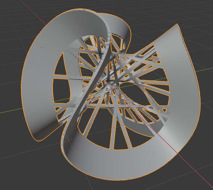
To make an .stl file, all that’s left to do is surface.save('path/to/file.stl'). Since this object has no thickness, it is not yet suitable for 3D printing. We first used Blender to solidify the mesh, resulting in something like this:

We sent the .stl file for the thickened surface to the Form 2 printer at the University of Kentucky Math Lab, and after a 23 hour print and some careful support clipping, this was our final product:

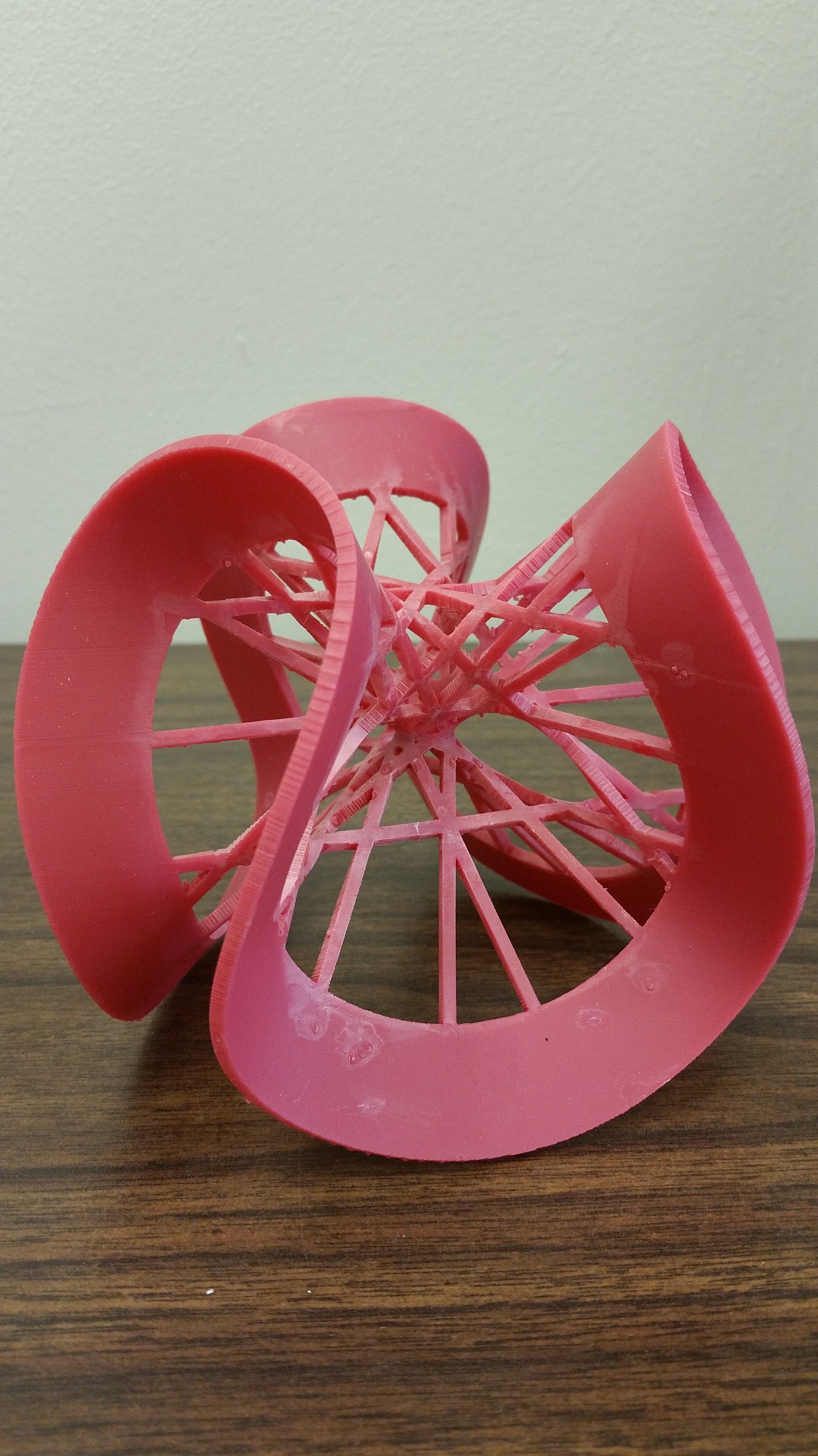
We’re quite happy with the results, since it accentuates the pieces of the surface that contain straight lines, while still showing the local twisting of the surface around those lines. This model now has a home in the display case in the math department at UK.