N Fieldsteel

Langton's ant part III - Visualizations with OCaml

A few years ago I gave a talk to Kentucky’s undergrad math club about cellular automata, and I summarized that talk in a two-part blog post on this site. Here are links to part I and part II. At the end of the second post I mentioned that I had made videos using Ryan Wick’s Langton’s Ant Animator, but that I wanted to try making my own videos with my own code from the ground up. I just wrapped up this project. You can see the final result below, which I suggest watching fullscreen and in 4K resolution if possible.

Code

Here is the github repo for the code I wrote. Keep in mind that while it’s usable, I didn’t write it with users other than myself in mind. So it’s not particularly friendly. See the readme on github for instructions on how to compile and use it.

Motivations

As I mentioned in earlier posts, part of my motivation for this project came from Ryan Wick’s video and his Langton’s Ant Animator. Why did I start this project when something similar has already been done with freely available source code? A few reasons:

• Langton’s Ant is simple. There’s very low overhead to implement it from scratch.
• I was mainly interested in making images where each pixel of the image corresponds to a point in the ant’s grid. This is simpler than drawing a more general grid of squares, which further reduced the overhead of starting from scratch.
• I had my own ideas about automating the search for visually interesting examples, and implementing these ideas myself seemed easier than tweaking an existing codebase.
• When producing a video frame-by-frame, I wanted to allow the number of steps the ant takes per frame to vary, for aesthetic reasons discussed below.

High-level summary

The project was straightforward, especially because I had an existing codebase to use as a roadmap. My plan was

1. Implement Langton’s Ant.
2. Implement writing and saving images that show the ant’s current state.
3. Write and save the images that correspond to the frames of an animation.
4. Stitch those frames into a video with ffmpeg.

Code

Basic types

The grid we’ll use is just a \(2\)-dimensional array of integers. In theory it’s infinite, like the tape of a Turing machine. In practice it just needs to be big enough that we don’t need to worry about reaching the edge.

type grid = int array array

The position of the ant is a \(2\)-tuple of ints representing its location in the grid. The direction of an ant is also a \(2\)-tuple of ints, representing the direction vector we’ll use when we update the ant’s position.

type position = int * int

type direction = int * int

A turn is one of the four ways the ant’s direction can change when it reaches a new square,

type turn =
  | Left
  | UTurn
  | Right
  | Straight

and an ant’s rule is just an array of turns

type rule = turn array

So for us, the classic rule RL is the OCaml array [|Right; Left|]. Finally, an ant is a record type consisting of a rule (which never changes) as well as a position and a direction, both of which can change.

type ant = {
    rule : rule;
    mutable position : position;
    mutable direction : direction;
  }

To maintain the entire state of an ant’s run, we’ll use another record type. In essence a state is just an ant and a grid. But in practice we’ll carry along a bit more data, some for convenience and some with a mind towards our image-related needs in the future. For us, a state is an ant, a grid, as well as the dimensions of the grid, an Rgb24.t image, the dimensions of that image, and the number of colors the ant uses.

type state = {
    colors : int;
    grid_width : int;
    grid_height : int;
    grid : grid;
    ant : ant;
    img_width : int;
    img_height : int;
    img: Rgb24.t
  }

The reason for maintaining the grid and the Rgb24.t image simultaneously may not be the best design choice, but my reasoning was as follows. We really only care about images of size \(3840 \times 2160\) for making 4K video. But if an ant starts in the middle of such an image and follows its rule for a while, it might leave that bounded region and return later. In practice this happens quite often. So I decided to maintain a larger grid of integers, the center of which corresponds to the 4K image. This is less memory intensive and easier to work with than maintaining an enormous image then throwing most of it out at the end.

When the ant takes a step, two things happen:

1. The state’s ant and grid are updated appropriately.
2. If the ant’s position places it in the portion of the grid that corresponds to the Rgb24.t image, then the image is also updated.

Basic functions

Next we need a few functions for updating the state. For example, we can rotate ant a through turn t by updating the ant’s direction.

let rotate t a =
  let (u,v) = a.direction in
  match t with
  | Left -> a.direction <- (v, -u)
  | UTurn -> a.direction <- (-u, -v)
  | Right -> a.direction <- (-v, u)
  | Straight -> a.direction <- (u, v)

and we can move an ant by updating its position using its direction vector.

let move a =
  let (i,j) = a.position in
  let (u,v) = a.direction in
  a.position <- (i + u, j + v)

Checking whether or not position (i,j) is in the Rgb24.t image of a given state just requires a few inequalities.

let in_img i j s =
  let gw = s.grid_width in
  let gh = s.grid_height in
  let iw = s.img_width in
  let ih = s.img_height in
  
  (gw - iw) / 2 <= i
  && i < iw + (gw - iw)/2
  && (gh - ih) / 2 <= j
  && j < ih + (gh - ih) / 2

And given position (i,j) in the grid of state s we can find the coordinates of the corresponding point in the Rgb24.t image.

let img_coords i j s =
  let gw = s.grid_width in
  let gh = s.grid_height in
  let iw = s.img_width in
  let ih = s.img_height in
  (i - ((gw - iw)/2),
   j - ((gh - ih)/2))

Now given a state s we can have the ant change the color of the square it’s on. First it updates the grid. Then if necessary it also updates the image.

let change_color s =
  let (i,j) = s.ant.position in
  let color = s.grid.(i).(j) in
  let next_color = if color = (s.colors - 1)
                   then 0
                   else color + 1 in
  s.grid.(i).(j) <- next_color;
  if in_img i j s
  then (let (p,q) = img_coords i j s in
        Rgb24.set s.img p q color_list.(next_color))
  else ()

In the code above, color_list is a list of n random colors, where n is the length of the rule to be used and the first color is always #000000. It is generated at runtime when the user specifies a rule of length n.

When we update the state by allowing the ant to take a step, we check whether the ant is still within the confines of the grid. If it is, we rotate, change_color, and move. If it’s not, then we do nothing. This is a little lazy and would be better handled with exceptions. But for a project of this scope I think some laziness is fine.

let step s =
  let (i,j) = s.ant.position in
  let gw = s.grid_width in
  let gh = s.grid_height in
  if (0 <= i && i < gw && 0 <= j && j < gh)
  then (let c = s.grid.(i).(j) in
        let t = s.ant.rule.(c) in

        rotate t s.ant;
        change_color s;
        move s.ant)
  else ()

To take i steps we make use of some of the imperative features of OCaml.

let steps i s =
  for j = 1 to i
  do
    step s
  done

Saving images

With the CamlImages library, saving the Rgb24.t image of state s to a file with filename fname is straightforward.

let save_image fname s =
  let output = Images.Rgb24 s.img in
  Images.save fname (Some Png) [] output

Making animation frames

In making the frames of an animation, we arrive at one of the main reasons why I chose to code this up from scratch: Many of the most visually interesting examples I could find seemed to build and fill in an expanding square. In my mind, an animation showing such an ant looks best if the square grows at a constant rate. But when the ant takes a constant number of steps per frame, the square’s growth will appear to slow over time. But for these expanding-square examples, if the ant takes \(b \cdot i\) steps during frame \(i\) where \(b\) is some constant, the growth of the square will appear roughly constant. This is only a heuristic, since even if the ant does build an expanding square, its precise behavior is more complicated and less predictable. But in practice this seems to work quite well. We just need to find the conatnt \(b\), which takes some easy algebra.

Say you want to make a \(15\)-second long animation where an ant takes 100_000_000 steps. For \(15\) seconds you’ll need 900 frames. If the number of steps taken by the ant per frame is fixed, that would mean 100_000_000 / 900 = 111111 steps each frame. But if the ant is taking \(b\cdot i\) steps per frame, we need

\[\sum\limits_{i = 0}^{900} b\cdot i = 10^{8}\]

But the left hand side simplifies:

\[b\cdot \frac{(900)(901)}{2} = 10^8\]

which means

\[b = \frac{2 \cdot 10^8}{(901)(902)} = 246.\]

This means that between frame 0 and frame 1, the ant takes 246 steps. Between frames 1 and 2 the ant takes 2 * 246 steps, and so forth, At the beginning of the animation the ant is taking far fewer than 111111 steps per frame. This slows down the beginning of the animation. At the end of the animation the ant is taking significantly more than 111111 steps per frame, which speeds up the end of the animation.

If you already know the rule, the number of frames num_frames to generate, and the number of steps num_steps to take, here’s how you could generate the save the frames of a smooth animation.

This creates a directory named rule, then moves into that directory and saves all the relevant images with sequential integers as filenames. Finally, it makes a system call to ffmpeg to stitch the frames together into a video.

let animation_frames gw gh iw ih =
  let s = num_steps in
  let f = num_frames in
  let coeff = 1 + (2 * s) / (f*f + f) in
  let frames i = coeff * i in
  Sys.mkdir rule 0o777;
  let fn_length = f
                  |> float_of_int
                  |> log10
                  |> Float.floor
                  |> (+.) 1.
                  |> int_of_float in
  let filename i =
    let num = string_of_int i in
    let k = String.length num in
    "00"^(String.make (fn_length - k) '0') ^ num in
  let state = initialize_state ~gw:gw ~gh:gh ~iw:iw ~ih:ih rule in
  save_image (rule ^ "/" ^ (filename 0) ^ ".png") state;
  for j=1 to f
  do
    steps (frames j) state;
    save_image (rule ^ "/" ^ (filename j) ^ ".png") state;
  done;
  Sys.chdir rule;
  ignore (Sys.command ffmpeg_call);
  Sys.chdir "..";;

In the code I wrote, ffmpeg_call is a string, depending on the rule, given by:

let ffmpeg_call = "ffmpeg"
                  ^ " -f image2"
                  ^ " -pattern_type glob"
                  ^ " -framerate 60"
                  ^ " -i '00*.png'"
                  ^ " -s 3840x2160"
                  ^ " " ^ rule
                  ^ ".mp4"

But this can be tweaked or removed as needed.

Notes on performance

When I was writing part II of this post, I wrote a naïve implementation of Langton’s Ant in Mathematica. I revisited that implementation now, and ran the rule RLLR on a grid of size \(10,000 \times 10,000\) for \(2,000,000\) steps. There was no image writing or even image displaying, just updating a SparseArray. The computation took 83.9 seconds. By contrast, my naïve OCaml implementation outlined above ran the same computation in .08469 seconds. That’s close to \(1000\) times faster. I am certain that the Mathematica implementation can be improved, though making performance optimizations to Mathematica code can be complex and somewhat arcane. There are likely some improvements that could be made to my OCaml implementation too. But in this case all I care about is comparing my naïve first-pass implementations, and here OCaml is the clear favorite.

It’s also worth considering the performance impact of updating the Rgb24.t image every time the ant takes one step. It’s of course possible that the ant will change the same pixel many times between calls to save_image, and it’s not important to perform all those updates to the image. Could it be better to just build the entire image from scratch using the data in the grid every time you want to write an image file? The answer is that this might be better in theory, but in practice this was never the case.

Say you’re working with an image of size \(w \times h\). Would you rather update all \(w\cdot h\) pixels of the image using data from the grid, or would you prefer to update \(s\) pixels of an existing image, where \(s\) is the number of steps the ant is going to take? The answer depends entirely on whether \(s\) is bigger or smaller than \(w \times h\), and for the purposes of making the 4K videos you see above, \(s\) was always smaller by several orders of magnitude.

Searching for visually interesting rules

To find rules worth animating, I did some fairly exhaustive searches of short rules consisting of only L and R. By symmetry, it’s enough to consider just the rules that start with R, which cuts the search space in half. Additionally, you can safely ignore cyclic strings (a cyclic string is a string s that’s of the form t ^ t ^ ... ^ t for some shorter string t). An ant with rule RRLRRL or RRLRRLRRL will follow the exact same path as the ant with rule RRL, for obvious reasons.

So the number of rules of length \(n\) is just half of the \(n^{\text{th}}) term of OEIS sequence A027375, which grows pretty fast. But it was completely feasible to generate all rules of length \(13,14\) and \(15\), run each ant for \(50\) million steps or so, and save all the resulting images.

That took about a day and gave me a nice starting point in the search for interesting examples. What I quickly noticed is that rules that shared a long prefix tended to produce similar-looking patterns. It’s easy to guess at some heuristic justifications for why this ought to be the case, but it’s not a universal rule. Even when stated this informally, it admits plenty of counterexamples.

But in practice it means that if I found a rule string \(r\) that made a somewhat interesting pattern, and I wanted to see some variations on that theme, I could then inspect the associated rules

\[\{r \wedge s~|~ \text{len}(s)\leqslant k\},\]

for small values of \(k.\) Among these rules I would often (but not always) find lots of examples of similar-looking patterns, and I could select the one which filled space the fastest, or which had the most structure and the least noisy chaos. If none of them were satisfactory I could pick a few favorites and iterate, or I could increase \(k\) and try again.

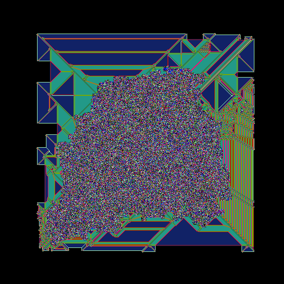
For example, I was interested in the length \(13\) rule RLRRLLLLLLLLL, for which my code had generated this preview.

But the larger animation was unsatisfying. After searching, I thought the length \(15\) rule RLRRLLLLLLLLLRR was promising. Its preview looked like this:

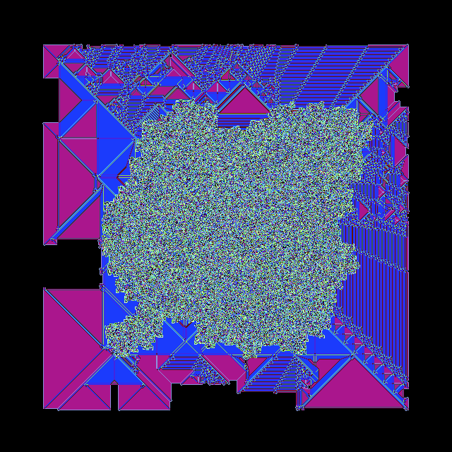
It has many features and behaviors in common with the original rule, but it seemed to fill space a bit faster and I thought it would make a better visualization. But the final animation was also not great. Eventually I found the length \(18\) rule RLRRLLLLLLLLLRRLLL with preview:

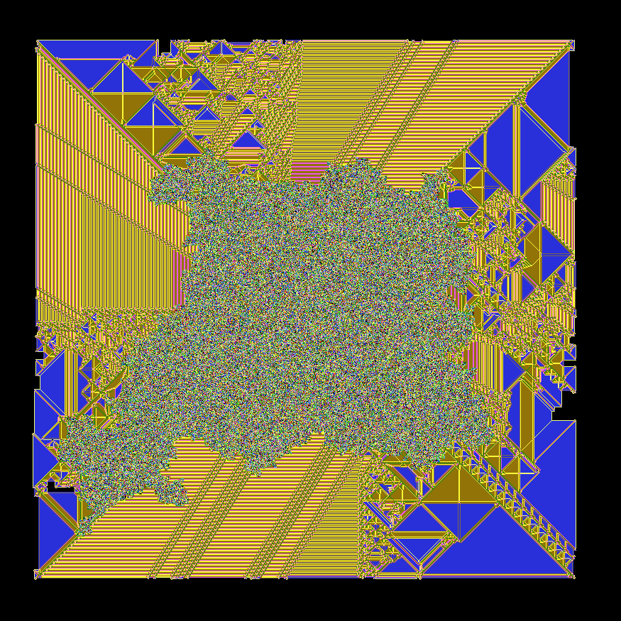
And this is the one that made it into the final video. You can see it at 1:27.

Future directions

I would like to extend my code to handle more general turmites and make a second video. I don’t see any technical hurdles, it should be straightforward. But that’s a project I’ll save for another day.