N Fieldsteel

3D Printing a Permutoassociahedron

In this post, we’ll put together a 3D-printable model of a permutoassociahedron. Along the way we’ll also get models of some related polytopes. The code, illustrations and models produced here are my own. The mathematical underpinnings of this post are secondary polytopes and fiber polytopes, and the constructions I used came from the existing literature. Detailed descriptions of these constructions, along with significantly more background, detail, and proofs, can be found in the papers listed at the bottom of this post.

Introduction: face lattices of polytopes.

Consider a triangle with vertices \(a,b\) and \(c.\)

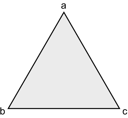
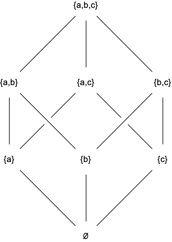
This triangle gives rise to a partially ordered set in a natural way: The triangle itself contains \(3\) edges. Each edge contains \(2\) of the vertices. And each vertex contains the empty set. This triangle is a very simple example of a convex polytope, and this eight-element poset is called the face lattice of the polytope. The Hasse diagram of the face lattice looks like this.

Of couse, taking the face lattice of a convex polytope is not the only way to build a poset. Posets show up all the time in algebra, combinatorics, geometry, topology, and elsewhere. And not every poset can be realized as the face lattice of a convex polytope. When you’re given a poset, somtimes it’s possilble to find an ad hoc construction of a convex polytope whose face lattice is the specified poset. Or sometimes you can prove the existence of such a polytope but lack an explicit construction, or lack a particularly clean or symmetric construction.

In this post, we’ll talk about a few classes of combinatorially-determined posets for which corresponding convex polytopes are known to exist, admit very nice descriptions, and can easily be visualized or even 3D printed.

First example: the permutohedron

A permutation of a set \(X\) is usually defined as a bijection \(\sigma : X \rightarrow X.\) The six permutations of \(X=\{a,b,c\},\) written in one-line notation, are

\[abc\hspace{1.5em}acb\hspace{1.5em}bac\hspace{1.5em}bca\hspace{1.5em}cab\hspace{1.5em}cba.\]

But we can also think of a permutation as a choice of total ordering of \(X,\) where for example the permutation \(bac\) corresponds to the choice of total ordering \[b<a<c.\]

The appeal of this perspective is that it admits a natural generalization. If we say \(“b\) is smallest, \(a\) is in the middle, and \(c\) is largest”, then we’ve specified exactly the permutation \(bac\) above. But if instead we only say “\(b\) is smallest”, this does not specify a total order on \(X,\) so it doesn’t determine a permutation of \(X.\) But we can think of it as an “incomplete” total ordering on \(X.\) There are only two total orderings of \(X\) where \(b\) is the smallest element, and they correspond to the permutations \(bac\) and \(bca.\)

More formally, instead of considering only the total orderings on \(X,\) we consider the set of all strict weak orderings of \(X.\) A strict weak ordering on \(X\) is a total ordering of a partition of \(X.\) We’ll use the standard notation for strict weak orderings. For example, with \(6\) elements we would write \(b|adf|ce\) to mean the strict weak ordering \[\{b\}<\{a,d,f\}<\{c,e\}.\] The total orderings of a set \(X\) correspond to the strict weak orderings of \(X\) where the cells of the underlying partitions are singleton sets.

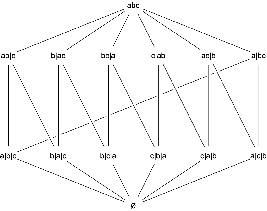
The set of strict weak orderings of \(X\) is partially ordered by refinement. When \(\nobreak{X=\{a,b,c\}},\) the poset of strict weak orderings of \(X\) (together with a smallest element, called \(\varnothing\)) looks like this.

We’d like to know whether this the face lattice of a convex polytope. By inspection, such a polytope would need to be \(2\) dimensional, and would need to have \(6\) vertices and \(6\) edges. The only candidate is a hexagon, and it’s easy to confirm that this poset is indeed the face lattice of a hexagon. Here’s a hexagon with its faces labelled to make the correspondence explicit.

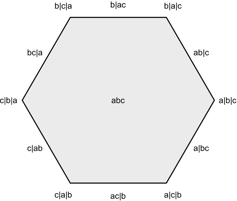
This is the \(2\)-dimensional permutohedron, a polytope whose vertices correspond to permutations and whose face lattice is the poset of strict weak orderings. But labelling a regular hexagon was just a one-off construction that works for the case when \(X\) has \(n = 3\) elements. In the \(n = 4\) case, the poset is significantly more complicated, having \(76\) elements instead of just \(14,\) and it’s much harder to find an ad-hoc construction of a corresponding polytope.

But it turns out there’s a straightforward construction that works for all \(n.\) Let \(\mathcal{V}\) be the set of vectors obtained by permuting the entries of the vector \(\langle 1,2,\ldots, n\rangle,\) i.e. \[\mathcal{V} = \{\langle\sigma(1), \sigma(2), \ldots, \sigma(n) \rangle: \sigma \in S_n\}.\]

The convex hull of \(\mathcal{V}\) lies in a codimension \(1\) affine subspace of \(\mathbb{R}^n,\) and is an \((n-1)\)-dimensional convex polytope whose face lattice is exactly the poset of strict weak orderings of an \(n\) element set. In the \(n=4\) case we can get a nice visualization with Mathematica.

V = Permutations[{1, 2, 3, 4}];
r = RotationMatrix[{{1, 1, 1, 1}, {0, 0, 0, 1}}];
Table[(r . v)[[;; 3]], {v, V}] // ConvexHullMesh

Which leads us to this visualization of the \(n=4\) permutohedron.

All that’s left to do is to make explicit the correspondence between the vertices of this convex hull and the strict weak orderings as above, but this is straightforward. In general, the vertex \(\langle \sigma(1), \sigma(2), \ldots, \sigma(n) \rangle\) determines a total ordering of its indices by comparing entries. For example, consider the vertex \(\langle 2,4,3,1 \rangle.\) The \(4^{\text{th}}\) entry is smallest, followed by the \(1^{\text{st}},\) then the \(3^{\text{rd}},\) and finally the \(2^{\text{nd}}.\) So this vertex correspondes to the permutation \(4132.\) Under this vertex labeling, the convex hull above is the \(3\)-dimensional permutohedron.

Second example: the associahedron

Most people are familiar with associative binary operations. These are operations for which the placement of parentheses in an expression does not change the value of that expression. The usual examples are operations like addition and multiplication. \[(a+b)+c = a+(b+c)\] \[(ab)c = a(bc).\]

But there are many binary operations that are not associative, or that are only associative up to isomorphism or up to homotopy. And there are even some binary operations that are associative, but for which the placement of parentheses can significantly affect the difficulty of the intermediate computation despite not changing the final value of the expression. For example, matrix multiplication is associative but the placement of parentheses in a product of matrices can significantly effect the computational complexity of evaluating that product.

This leads us to consider the combinatorics of all the meaningfully different ways to parenthesize an algebraic expression involving \(n\) symbols. When \(n = 4\) you have expressions like \((a(bc))d\) and \((ab)(cd),\) but there are also incomplete parenthesizations like \(a(bcd)\) or just \(abcd.\) The set of all such expressions forms a poset, where the ordering is determined by whether one expression can be turned into another by adding or removing a matching pair of parentheses. The poset in the case of \(4\) symbols looks like this.

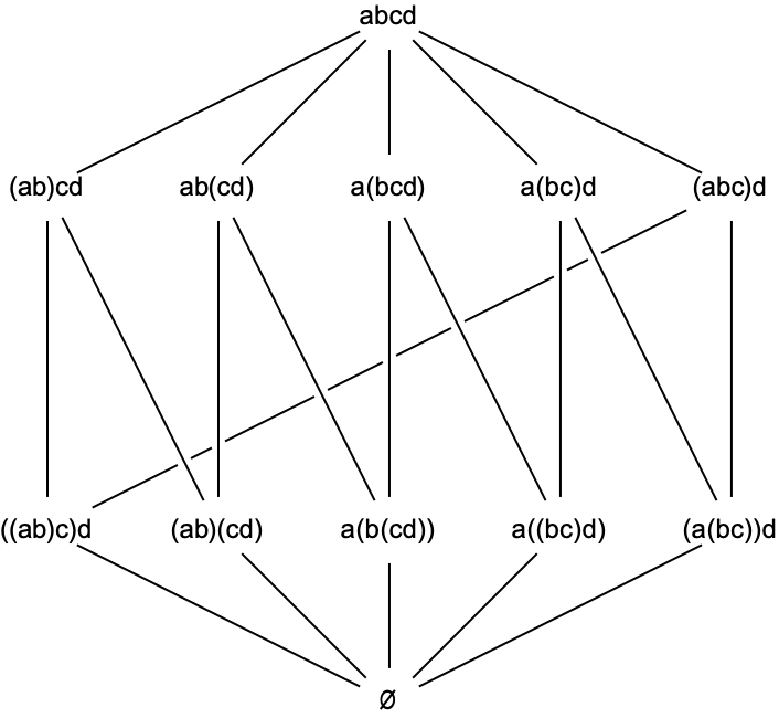
Just like with the permutohedron above, this poset is small enough that we can find by hand a convex polytope with this poset as its face lattice. Here it is.

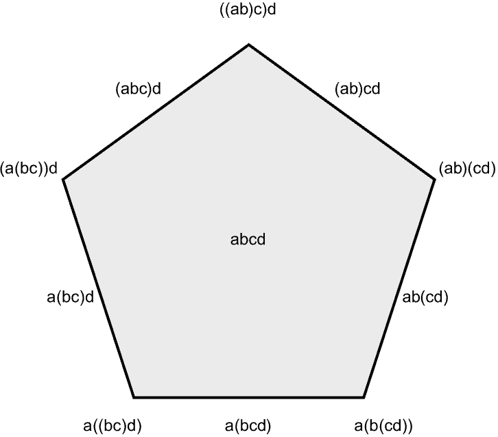
This pentagon is the \(2\)-dimensional associahedron. But once again, we’d like a general construction for higher-dimensional associahedra, especially for the dimension \(3\) case. It turns out there are a lot of different constructions, and many of them are described in detail here. The secondary polytope construction is best for our purposes.

To describe this construction, we first note that there’s a bijective correspondence between the set of complete parenthesizations of a string of \(n\) symbols and the set of triangulations of a regular \((n+1)\)-gon. To see why, consider a string of \(n\) symbols and label the \(n+1\) locations where parentheses can be placed with the integers from \(1\) to \(n+1.\)

\[\underset{1}{\rule{.3cm}{0.1mm}}~a~\underset{2}{\rule{.3cm}{0.1mm}}~b~\underset{3}{\rule{.3cm}{0.1mm}}~c~\underset{4}{\rule{.3cm}{0.1mm}}~d~\underset{5}{\rule{.3cm}{0.1mm}}~e~\underset{6}{\rule{.3cm}{0.1mm}}\]

Then place corresponding labels on the vertices of a regular \((n+1)\)-gon. Now given a particular parenthesization, we can identify matched pairs of parentheses with diagonals in the \((n+1)\)-gon, under which a complete parenthesization corresponds to a triangulation. With a color-coded example, the expression \(\color{00ff00}{(}\color{ff0000}{(}\color{000000}{a}\color{000000}{b}\color{ff0000}{)}\color{000000}{c}\color{00ff00}{)}\color{0000ff}{(}\color{000000}{d}\color{000000}{e}\color{0000ff}{)}\) corresponds to the triangulation of the hexagon shown here.

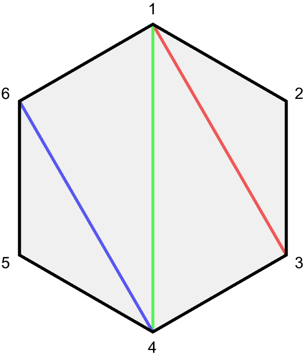
For a given triangulation \(T\) of this hexagon, consider the point \(v(T) = \langle a_1, \ldots, a_6 \rangle,\) where \(a_i\) is the sum of the areas of the triangles in \(T\) that have vertex \(i\) as a corner. If \(\mathcal{T}\) is the set of all triangulations of this hexagon, let \(V\) be the set \(\left\{v(T):T\in \mathcal{T}\right\}.\) \(V\) lies in a \(3\)-dimensional affine subspace of \(\mathbb{R}^6.\) Using an orthonormal basis to get \(3\)-dimensional coordinates for that space will embed these points in standard \(\mathbb{R}^3.\) It turns out these points will be the vertices of a \(3\) dimensional associahedron.

Enumerating all triangulations of an \(n\)-gon requires a little thought. When \(n\) is small, there are few enough triangulations of of \(n\)-gon that we could just write them down by hand. But there is a nice recursive function, so we opt for that instead. The key insight is that for any triangulation \(T,\) the edge from \(1\) to \(n\) must be the edge of some triangle in \(T,\) say \(\{1,d,n\}\) for some \(d.\) Then we triangulate the the polygon with vertices \(\{1, \ldots, d\}\) and \(\{d, \ldots, n\},\) and concatenate. Ad \(d\) varies, this produces all triangulations of the \(n\)-gon without repetitions.

triangulations[v_]:=
   If[Length[v]<3,{{ }},
   If[Length[v]==3,{{v}},
      Flatten[Table[Join[t1,{{v[[1]],v[[d]],v[[-1]]}},t2],
      {d,2,Length[v]-1},
      {t1,triangulations[v[[;;d]]]},
      {t2,triangulations[v[[d;;]]]}],2]]]

Now we’re ready to follow the recipe outlined above to construct the associahedron. Let H be the set of vertices of a regular hexagon, and T the set of triangulations of H

H = {Re@#, Im@#}&/@Table[Exp[2 Pi I k / 6],{k, 1, 6}];
                            
T = triangulations[H];

For finding the area of a triangle, we use Heron’s formula.

len[i_, j_] := Norm[j - i];
heron[a_, b_, c_] := 
  Module[{s},
  s = (a + b + c)/2;
  Sqrt[s (s - a) (s - b) (s - c)]];
area[{i_, j_, k_}] := heron[len[i, j], len[i, k], len[j, k]];

We needed area for our v function, which is exactly \(v(T)\) described above.

v[t_] := Table[area /@ Select[t, MemberQ[i]] // Total, {i, H}];

Finally, V6 is the set of coordinates in \(\mathbb{R}^6,\) translated to contain the origin. B is an orthonormal basis for the subspace they span, and V3 is this set written with respect to B. We take the ConvexHullMesh to see the polytope.

V6 = v[#] - v[T[[1]]] & /@ T;
B = Select[Orthogonalize[V6 // N], Norm[#] > 0.1 &];
V3 := Table[Table[v . b, {b, B}], {v, V6}];

ConvexHullMesh[V3]

Here’s our \(3\)-dimensional associahedra, realized as the secondary polytope to a regular hexagon.

It’s worth noting that this polytope depends on exactly which hexagon you start with. If you don’t use a regular hexagon, this construction will give you a combinatorially equivalent polytope that’s not congruent to the one above. For a very nice visualization of how the associahedron changes as H is allowed to vary, see this excellent interactive visualization.

Permutoassociahedra

The permutohedra are convex polytopes that parametrize the different permutation of \(n\) symbols, while the associahedra parametrize the different ways to parenthesize a string of \(n\) symbols. If we instead consider all the ways to permute and parenthesize a set of \(n\) symbols, we’ll end up with a permutoassociahedron. The vertices of the permutoassociahedron correspond to complete parenthesizations of strings of symbols, and there’s an edge between two vertices exactly when you can get from one expression to the next using the associativity rule once, or by two swapping adjacent symbols that are grouped together by parentheses.

The full face poset of the \(n\)-dimensional permutoassociahedron is called the Kapranov poset. Its elements are parenthesizations of strict weak orderings of \(n+1\) symbols, where the \(|\) delimiter is treated like a binary operation and the contiguous blocks of symbols between delimiters are treated like atomic expressions. The precise definition of the ordering on these elements is a little fiddly to describe, so we’ll omit the full description here and jump straight into the construction. A complete description of this poset can be found here or here.

The construction is uses the theory of fiber polytopes. This particular construction is from the Coxeter Associahedra paper.

Consider a pentagon with vertex labels \(\{0,1,2,3,4\}.\) Let \(\mathcal{T}\) be the set of all triangulations of this pentagon. Its elements are triples of triples of indices defining valid triangulations, such as \[\left\{\{0,1,3\},\{0,3,4\},\{1,2,3\}\right\} \in \mathcal{T}.\]

Define \(f_i \in \mathbb{R}^4\) to be the vector which has \(1\) for the first \(i\) entries and \(0\) for the rest, and for a given triangulation \(T \in \mathcal{T},\) define

\[v(T) := \sum\limits_{T \in \mathcal{T}} \frac{1}{2}(j-i)(k-i)(k-j) (f_i + f_j + f_k).\]

The standard action of \(\sigma \in S_4\) on a vector \(w \in \mathbb{R}^4\) will be denoted \(\sigma\cdot w.\) With this notation, let \(V\) be the set

\[V = \{\sigma \cdot v(T) : \sigma \in S_4~\text{and}~T \in \mathcal{T}\}.\]

This set \(V\) is contained in a \(3\)-dimensional affine subspace of \(\mathbb{R}^4,\) and the convex hull of \(V\) is the \(3\) dimensional permutoassociahedron, a convex polytope whose face lattice is the poset mentioned above. The subspace containing \(V\) can be described as a set of points whose coordinates have a fixed sum, so identifying this subspace with \(\mathbb{R}^3\) only requires a simple rotation. In Mathematica, we can find the set V in \(\mathbb{R}^4\) as follors.

T = triangulations[Range[0, 4]];
f[i_] := Array[1 &, i]~Join~ Array[0 &, 4 - i];

v[T_] := Module[{summand},
   summand[{i_, j_, k_}] :=
    (j - i) (k - i) (k - j)/2 (f[i] + f[j] + f[k]);
   Sum[summand[t], {t, T}]];

V = Flatten[Table[Permutations[v[t]], {t, T}], 1];

Then we rotate V and drop the last entry of each vector to get coordinates in \(\mathbb{R}^3.\) We take the convex hull to see the polytope.

r = RotationMatrix[{{1, 1, 1, 1}, {0, 0, 0, 1}}];
V = Table[(r . v)[[1 ;; 3]], {v, V4}];
P = V // ConvexHullMesh

Here’s the final result.

Towards 3D printing

These constructions give us coordinates for the vertices of various convex polytopes in \(\mathbb{R}^3.\) The models above could be printed as is, but that would use a lot of plastic resin. It’s more efficient to instead 3D-print the \(1\)-skeleta of these polytopes. Making use of Mathematica’s MeshPrimitives functionality makes this very straightforward. In the function below, V is the set of vertices of the polytope in \(\mathbb{R}^3.\) We add an additional parameter r to control the thickness of the \(1\)-skeleton. The value of r is the desired ratio between the thickness of the \(1\)-skeleton to the length of the shortest edge in the \(1\)-skeleton.

oneskeleton[V_,r_]:=
Module[{n,t,edges,tube},
   t=r Min[Table[Norm[V[[j]]-V[[i]]],
           {i,1,Length[V]},
           {j,i+1,Length[V]}]];
   edges=MeshPrimitives[ConvexHullMesh[V],1];
   tube[Line[{p_,q_}]]:=Tube[{p,q},t];
   Table[tube[e],{e,edges}]//Graphics3D]

Because we already have explicit vertex sets for the three polytopes above, we get 3D-printable models immediately.

The associahedron:

The permutohedron:

And the permutoassociahedron:

References

• Coxeter Associahedra
• Many non-equivalent realizations of the associahedron
• The associahedron and triangulations of the \(n\)-gon
• Fiber Polytopes