The tangent variety to the twisted cubic
18 Feb 2020The twisted cubic curve is a famous example (and counterexample) in algebraic geometry, usually described parametrically as image of the map \(\vec{r} : \mathbb{P}^1 \rightarrow \mathbb{P}^3\) given by
\[ [s:t] \mapsto [s^3 : s^2 t : s t^2 : t^3],\]
though typically for visualization purposes, we’ll restrict our attention to the affine patch where \(s \not = 0,\) where we have the more familiar parametrization \(\vec{r} : \mathbb{R}^1 \rightarrow \mathbb{R}^3\) given by
\[\vec{r}(t) = (t, t^2, t^3).\]
Sean Grate and I were thinking about ideas for a 3D printed object that demonstrates something about the twisted cubic \(C.\) Right now we’re working on printing a model of the tangent variety to the twisted cubic which shows this surface as the union of of the tangent lines to the curve \(C\) itself.
To start, we’ll need parametric equations for the twisted cubic and it’s tangent vector. The model we’ll eventually be making will be bounded by the cube with vertices \((\pm 1, \pm 1, \pm 1),\) and we’ll be making this model out of cylindrical tubes of a fixed radius \(\epsilon,\) so we set up a region function and a choose a parameter accordingly.
r = {t, t^2, t^3};
v = D[r, t];

boundingcube = Function[{x, y, z},
   Abs[x] <= 1 &&
   Abs[y] <= 1 &&
   Abs[z] <= 1];
ep = 1/40;
For the twisted cubic itself, it’s straightforward to make a parametric plot.
curve = ParametricPlot3D[r, {t, -1, 1},
PlotRange -> {{-1.1, 1.1},
{-1.1, 1.1},
{-1.1, 1.1}},
PlotStyle -> Tube[ep],
RegionFunction -> boundingcube,
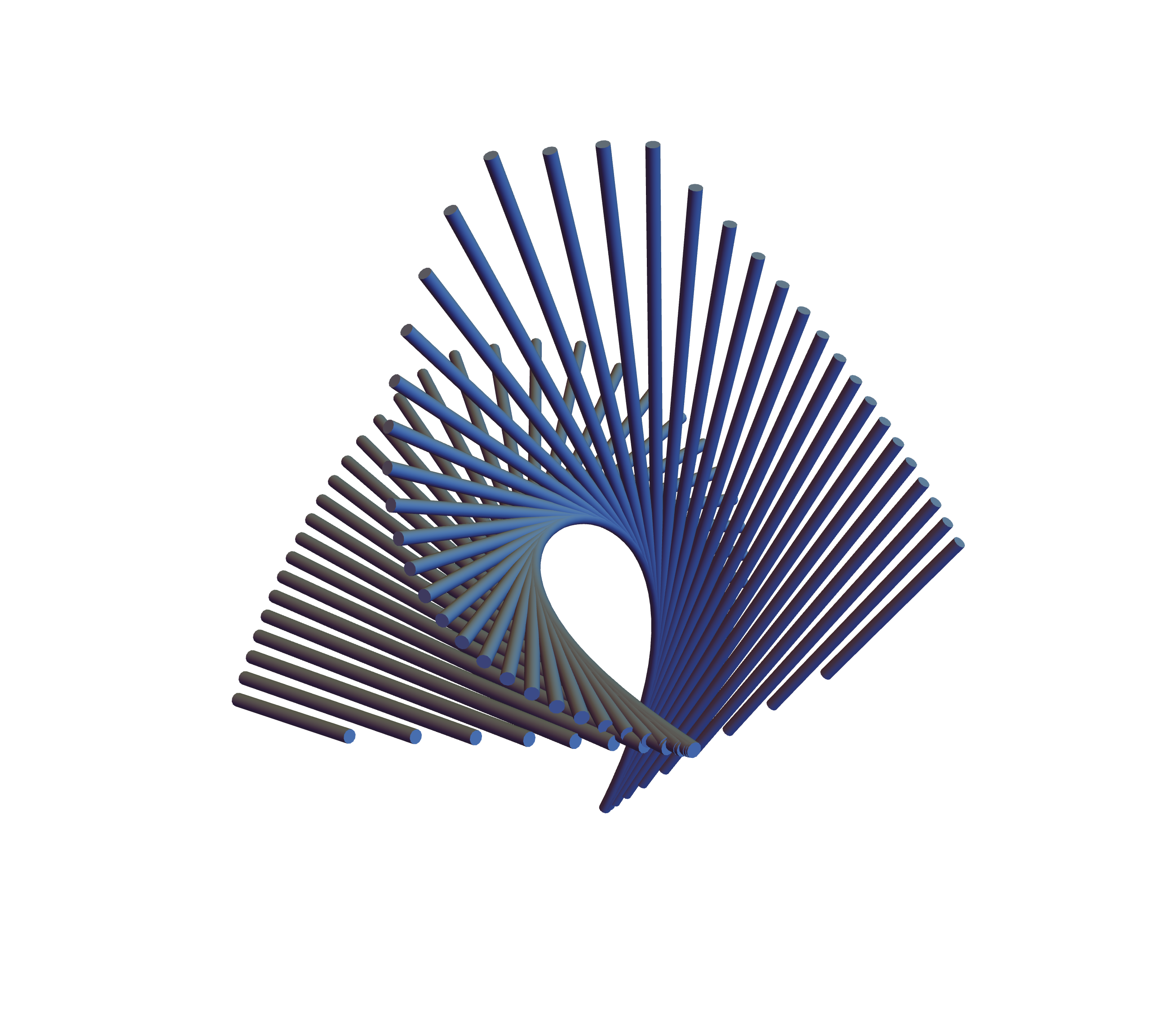
PlotPoints -> 50];Instead of plotting the tangent variety itself as a surface, we’ll instead plot a dense collection of tangent lines. For a fixed value of \(t,\) we get a tangent line to \(C\) is parametrized by
\[ \ell(s) = \vec{r}(t) + s \cdot\frac{d\vec{r}}{dt}(t).\]
We use this to create our collection of tangent lines.
tangents = Table[
   ParametricPlot3D[r + s v, {s, -5, 5},
    PlotRange -> {{-1, 1},
                  {-1, 1},
                  {-1, 1}},
    PlotStyle -> Tube[ep],
    RegionFunction -> boundingcube,
    PlotPoints -> 60],
   {t, -5, 5, 0.059}];
When we inspect what we have so far, we see that the curve together with this collection of tangent lines has some disconnected pieces, so it isn’t yet suitable for 3D printing.
Show[curve,tangents,Boxed -> False, Axes -> False]
To fix this, we’d like to add one more component to our model. We want to add the intersection of the tangent variety with the bounding box. Finding this intersection will be much easier if we know the implicit equation of the tangent variety, which we can get from the parametrization using Macaulay2. Our parametrization defines a ring map \(\mathbb{R}[x,y,z] \rightarrow \mathbb{R}[s,t],\) and the kernel of this ring map will be generated by the implicit equation of the tangent variety.
i1 : R = QQ[X,Y,Z];

i2 : S = QQ[s,t];

i3 : f = map(S,R,matrix {{t+s, t^2 + 2*s*t, t^3 + 3*s*t^2}});

o3 : RingMap S <--- R

i4 : ker f
             2 2     3      3             2
o4 = ideal(3X Y  - 4X Z - 4Y  + 6X*Y*Z - Z )

o4 : Ideal of R
To find the intersection of this surface with the faces of our bounding cube, we’ll set \(x,y\) or \(z\) equal to \(\pm 1,\) set the resulting expression equal to zero, and solve for one of the remaining variables.
tangentvariety = 3 x^2 y^2 - 4 x^3 z - 4 y^3 + 6 x y z - z^2;

face1 = Solve[(tangentvariety /. x -> -1) == 0, z] // Flatten;
face2 = Solve[(tangentvariety /. x -> 1) == 0, z] // Flatten;
face3 = Solve[(tangentvariety /. y -> -1) == 0, z] // Flatten;
face4 = Solve[(tangentvariety /. y -> 1) == 0, z] // Flatten;
face5 = Solve[(tangentvariety /. z -> -1) == 0, y] // Flatten;
face6 = Solve[(tangentvariety /. z -> 1) == 0, y] // Flatten;
What we get can be used to parametrize the different components of the intersection of the tangent variety with the bounding cube.
facecurves1 = Table[
   ParametricPlot3D[({-1, y, z} /. p), {y, -1, 1},
    PlotStyle -> Tube[ep],
    RegionFunction -> boundingcube,
    PlotPoints -> 40],
   {p, face1}];
facecurves2 = Table[
   ParametricPlot3D[({1, y, z} /. p), {y, -1, 1},
    PlotStyle -> Tube[ep],
    RegionFunction -> boundingcube,
    PlotPoints -> 40],
   {p, face2}];
facecurves3 = Table[
   ParametricPlot3D[({x, -1, z} /. p), {x, -1, 1},
    PlotStyle -> Tube[ep],
    RegionFunction -> boundingcube,
    PlotPoints -> 40],
   {p, face3}];
facecurves4 = Table[
   ParametricPlot3D[({x, 1, z} /. p), {x, -1, 1},
    PlotStyle -> Tube[ep],
    RegionFunction -> boundingcube,
    PlotPoints -> 40],
   {p, face4}];
facecurves5 = Table[
   ParametricPlot3D[({x, y, -1} /. p), {x, -1, 1},
    PlotStyle -> Tube[ep],
    RegionFunction -> boundingcube,
    PlotPoints -> 40],
   {p, face5}];
facecurves6 = Table[
   ParametricPlot3D[({x, y, 1} /. p), {x, -1, 1},
    PlotStyle -> Tube[ep],
    RegionFunction -> boundingcube,
    PlotPoints -> 40],
   {p, face6}];

facecurves = {
   facecurves1,
   facecurves2,
   facecurves3,
   facecurves4,
   facecurves5,
   facecurves6
   };
At the intersection points of these various facecurves, there’s a bit of artifacting we’d like to avoid, which we accomplish by covering these intersection points with a sphere of radius \(\epsilon.\) That way, the corners will be smooth instead of looking like two overlapping cylinders.
cornerpoints = {
   {-1, 1, -1},
   {1, 1, 1},
   {1, -1, 0.6569},
   {-1, -1, -0.6569},
   {1, 0.5408, -1},
   {-1, 0.5408, 1},
   {-0.5408, -1, -1},
   {0.5408, -1, 1}
   };

cornerdots = Table[
    Graphics3D[Sphere[p, ep]],
    {p, cornerpoints}];
The model we want is comprised of the twisted cubic curve, the collection of tangent lines, the curves of intersection between the tangent variety and the bounding cube, and these small corrective spheres.
components = {
	curve,
	tangents,
	cornerdots,
	facecurves
};

Show[components, Boxed -> False, Axes -> False]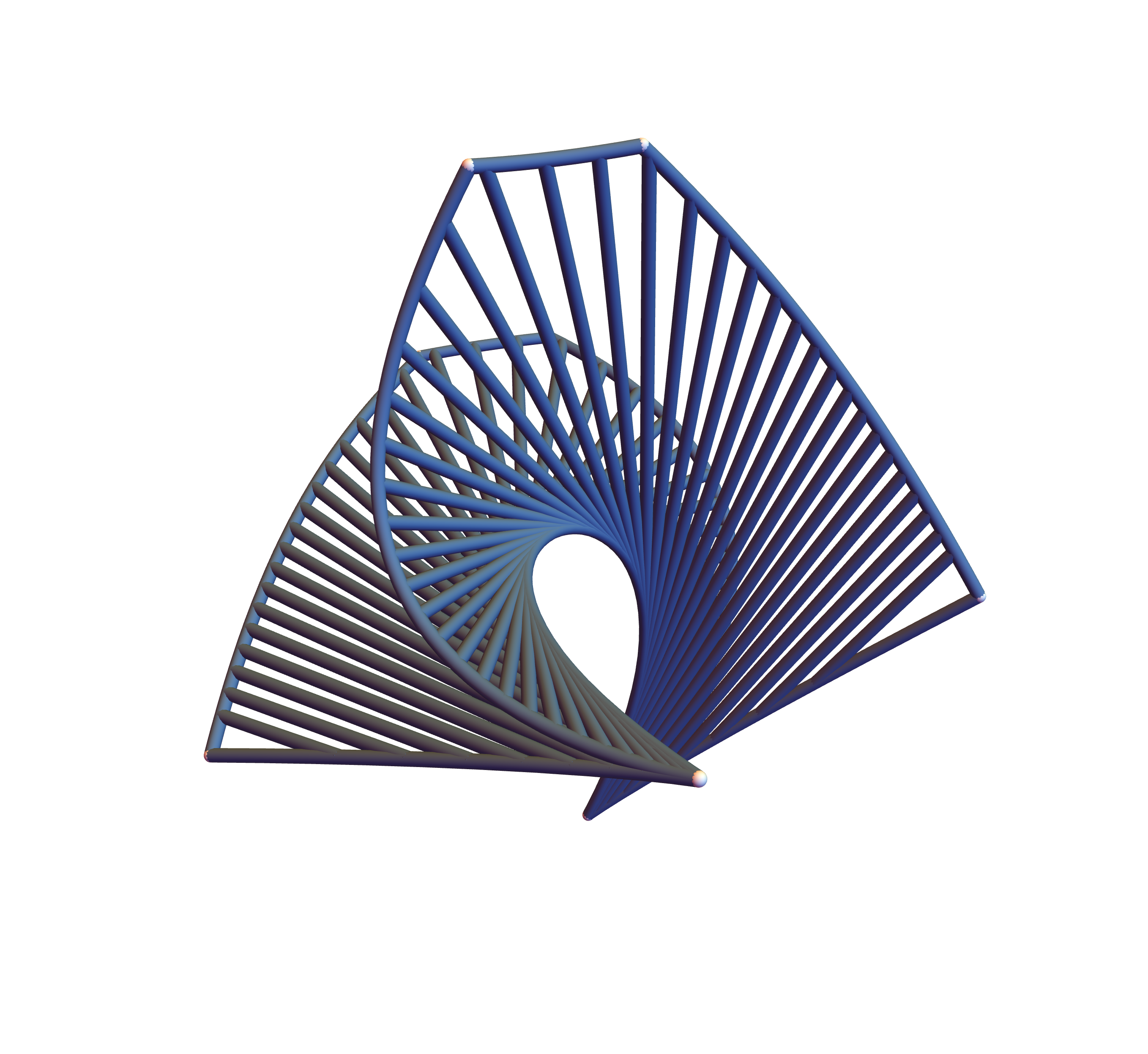
This can be exported to an stl file and 3D printed. (put picture here). It can be hard to understand what object looks like from a static picture, even a picture of a physical object. So for the purpose of this post, here’s a .gif made of a parametrized family of different views of the model.
frames = Table[
   Show[components,
   Boxed -> False,
   Axes -> False,
   ViewVector -> {3 Cos[t],
                  3 Sin[t],
                  6 Sin[t/2]}],
                  {t, 0, 4 Pi, 2 Pi/60}];

animation = ListAnimate[frames, 24];