N Fieldsteel

Cellular automata and Langton's ant - part I

Earlier this month I gave a talk at University of Kentucky Undergraduate Math Club about cellular automata and Langton’s ant. Here’s the poster the students made for the event.

The talk covered a few types of cellular automata at an introductory level and presented some nice visualizations. I’ll reproduce some of that exposition in a series of posts here, with a bit more detail about using Mathematica that I intentionally omitted from my talk.

Introduction

There are lots of examples of automata (singular: automaton) in math and computer science, so many that it’s difficult to find an all-encompassing definition that both gives clear intuition and is rigorous enough to work with. Essentially, an automaton is a mathematical model of a machine or process that is capable of doing some computation. Usually an automaton is thought of as some object that has various internal states. It periodically changes its state in a way that depends on its current state and possibly on some input. It may also produce some ouput based on its input and its internal state. In a precise definition this description would be formalized in the language of sets and functions. Probably the most well-known examples of automata come from the class of finite state machines, and include:

• Deterministic finite automata
• Pushdown automata
• Turing machines

Finite state machines are often introduced midway through a standard undergraduate computer science curriculum, usually alongside formal languages and maybe regular expressions. But my talk was not about these finite state machines. Instead, it was about a few conceptually simpler automata that are a bit further afield: cellular automata and Langton’s ant. In this post I will focus on cellular automata, saving Langton’s ant for the future.

Cellular Automata

The basics

A cellular automaton consists of a set of cells, each of which has its own state. The state of all of the cells is updated simultaneously according to a rule that takes into account the states of the cells and (usually) some structure on the set of cells. In most examples the cells are a \(1\) or \(2\) dimensional grid of squares, the states are colors, and the way an individual cell is updated depends on its state as well as the states of its neighbors.

One of the most well-known examples is Conway’s game of life, which is so well-known that for the relevant Google search the results page shows an animated game of life overlay. The cells are an infinite \(2\)-dimensional grid of squares, each of which is colored black or white, though these states are often referred to as “alive” or “dead”. To update the grid, we follow these two rules, where the “neighbors” of a cell are the \(8\) squares immediately adjacent to it.

1. If a cell is dead, it becomes alive if it has exactly three living neighbors. Otherwise it stays dead.
2. If a square is alive, it stays alive if it has exactly two or three living neighbors. Otherwise it dies.

These rules are simple, but they lead to some really complex behavior. I’ll leave a few links here.

• A small example.
• Some larger examples.
• A programmable computer.
• Game of life implemented in life.
• Brief interview with John Conway.
• And you can try it out yourself here.

But since my talk did not focus on Conway’s game of life, I won’t go into more detail. Instead, I’ll talk here about a class of even simpler cellular automata.

Elementary cellular automata

Elementary cellular automata consist of an infinite \(1\)-dimensional row of cells, where each cell is either black or white. The rule for updating a cell depends on that cell’s state as well as the state of its two neighbors. There are only eight possible configurations of the states of a cell and its neighbors, so to specify a rule we only need to make a decision about how to update a cell’s state in these eight cases.

Here’s an example of a rule we could follow to update the cells.

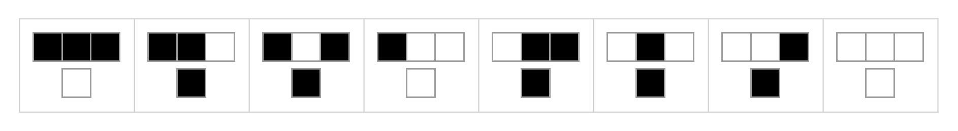
These eight choices can be identified with a binary string of length \(8\), i.e. with an integer from \(0\) to \(255\). For example, the rule above would be identified with the binary string \(01101110_2\), which is the decimal integer \(110\). Following the naming convention for cellular automata in Mathematica, this is “rule \(110”\). If we initialize the state of the cells so that exactly one cell is black and run this rule, what will happen? Well, here’s an animation that shows the first \(50\) steps.

But this isn’t really the most helpful way to visualize how the cells in this cellular automaton change over time. Instead, we’ll display a grid of cells, where the \(i^{\text{th}}\) row shows the state of the system after \(i\) steps. This is a standard way of visualizing these things, and it is straightforward in Mathematica.

ArrayPlot@CellularAutomaton[110, {{1}, 0}, 50]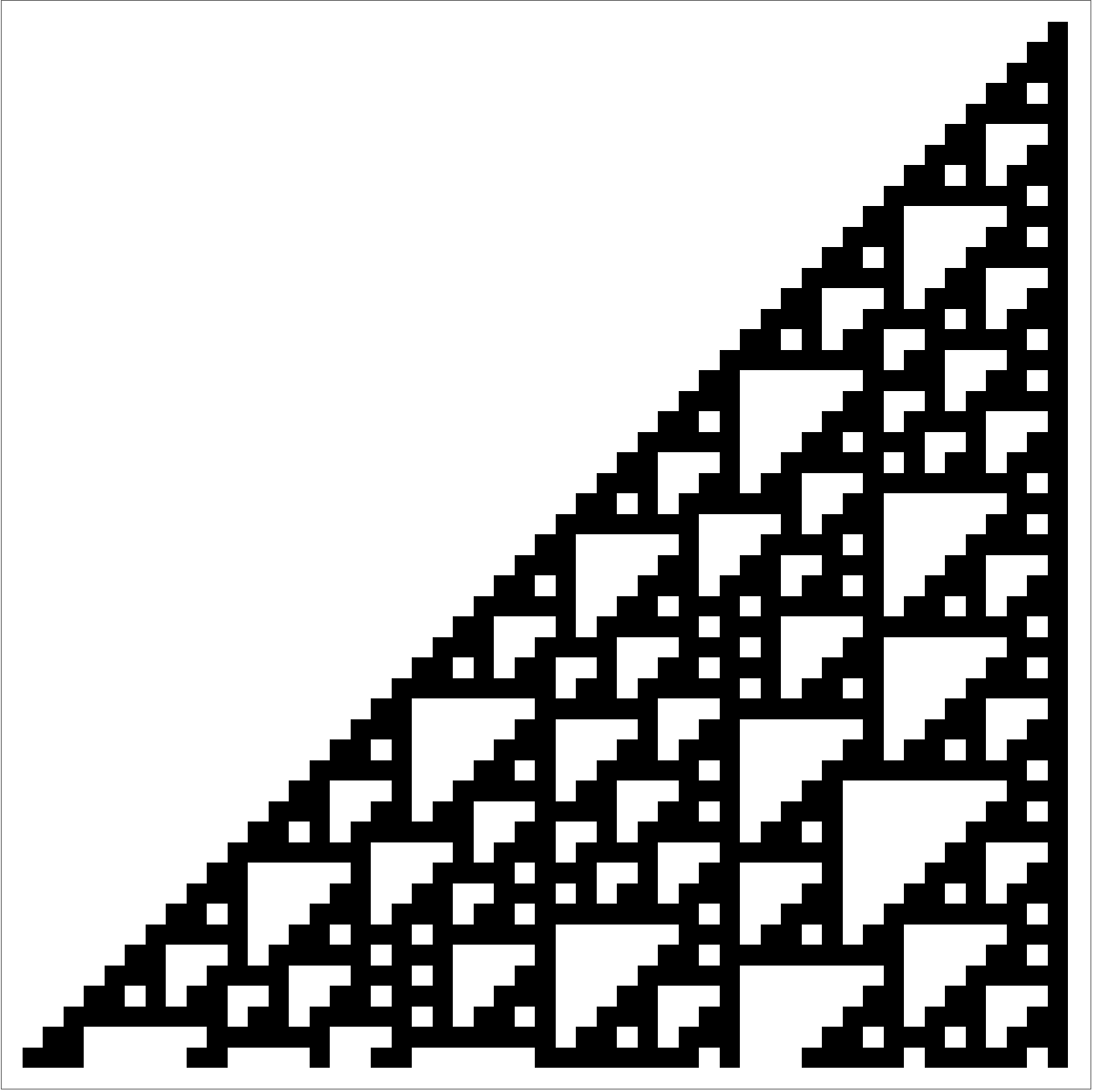

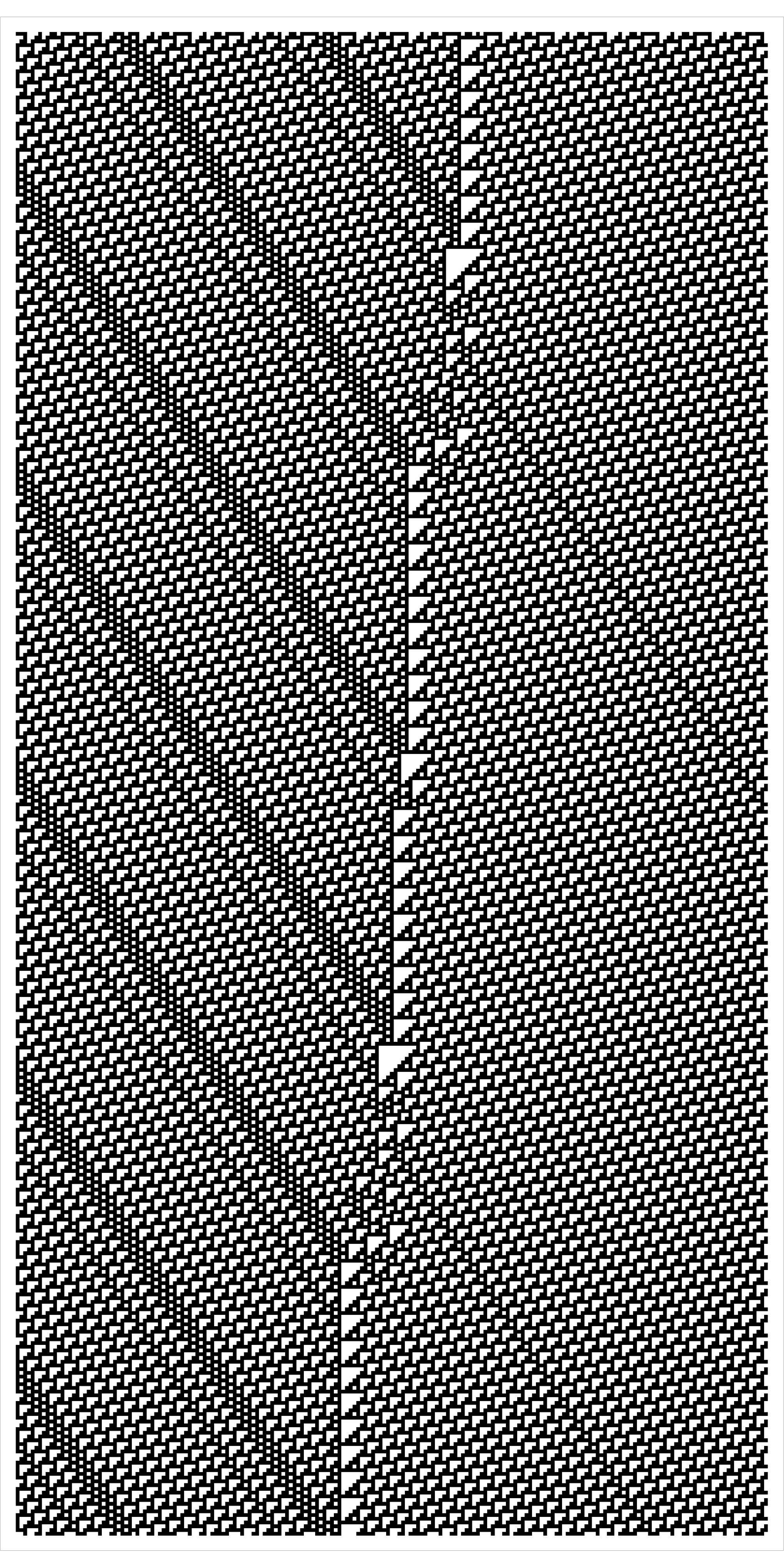
But this \(50 \times 50\) grid doesn’t really give me a good idea of the overall behavior. Is there a pattern? Some repetition? Let’s make a significantly bigger picture by showing not \(50\) but \(1500\) steps.

ArrayPlot[CellularAutomaton[110, {{1}, 0}, 1500], 
 PixelConstrained -> True,
 ImageSize -> {3000, 3000}]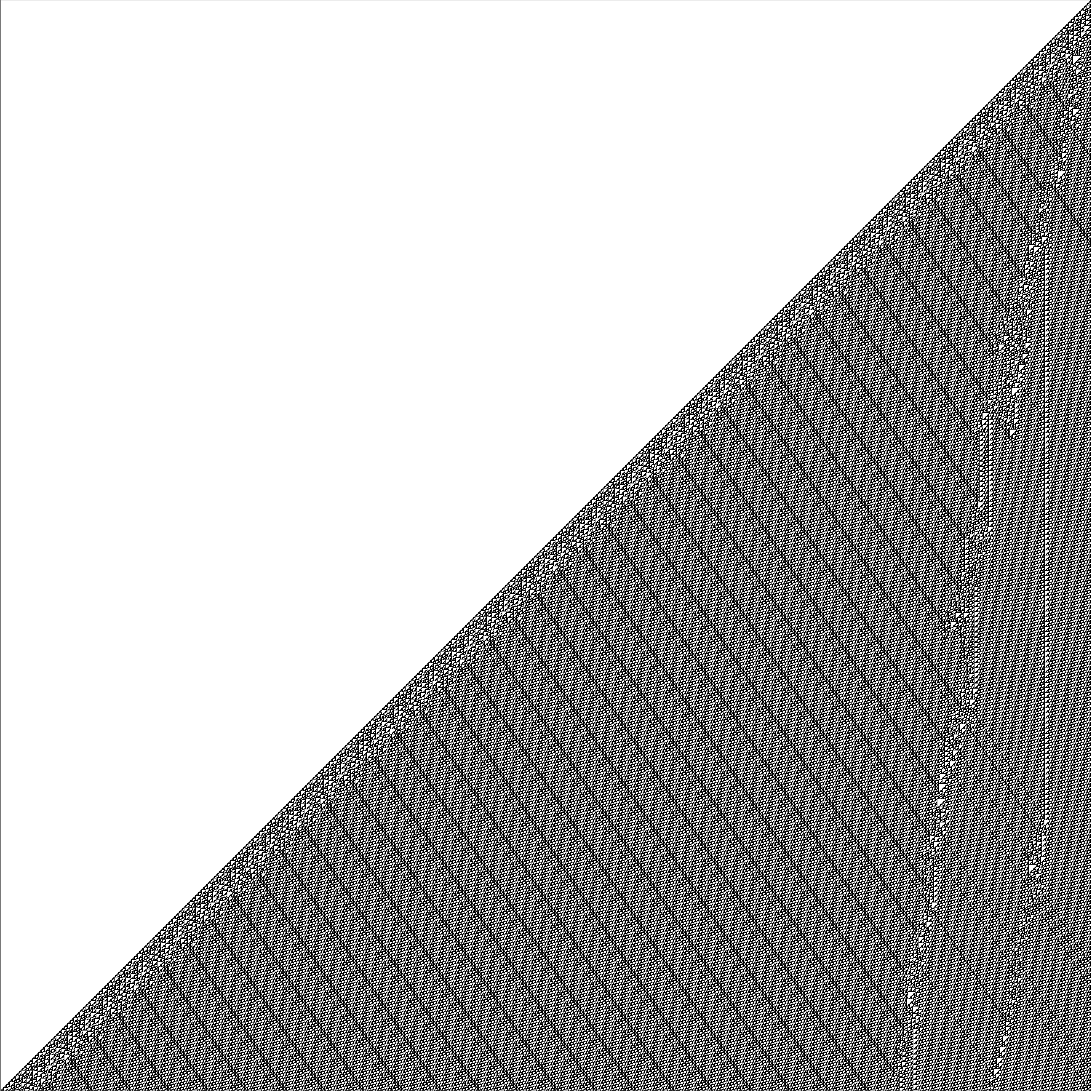

A good chunk of this image, comprising the leftmost edge of the triangle and most of its interior, seems to adhere to a predictable and regular pattern. But on and near the rightmost edge of the triangle this is not the case. There instead we see a non-pattern of apparently chaotic behavior.

This kind of dichotomy, where a simple rule produces both ordered and chaotic patterns, is a common feature of the automata I’ll talk about in this and future posts. Though I will note that, while the word “chaotic” is a commonly used descriptor of some of this behavior, I personally don’t feel that the word is a good fit. It suggests random or unpredictable behavior, which is not what we’re seeing here. Every pixel in this image is determined by the three pixels above it. We’re just following rule \(110\). Maybe “disorder” would be a better word than “chaos”.

Interestingly, the chaotic behavior on the right side of this image does not continue indefinitely. After around \(3000\) steps, all future rows adhere to a predictable, regular pattern. The eventual pattern you’ll see near the right edge of the triangle is this complicated (but repeating) motif, gradually drifting left.

The elementary cellular automata are fairly well-studied. Some, like rule \(0\), are completely trivial. Some, like our rule \(110\) above, exhibit more complex behavior that’s ultimately predictable and understandable (In fact rule \(110\) is known to be Turing complete). But some rules exhibit chaotic or disordered behavior and don’t appear to ever fall into a repetitive or predictable pattern. The most interesting of elementary cellular automata in this last class is probably rule \(30\).

Rule 30

Here is a visual representation of rule 30.

And jumping right into it, this is what happens after \(800\) steps, starting from an initial configuration of a single black square.

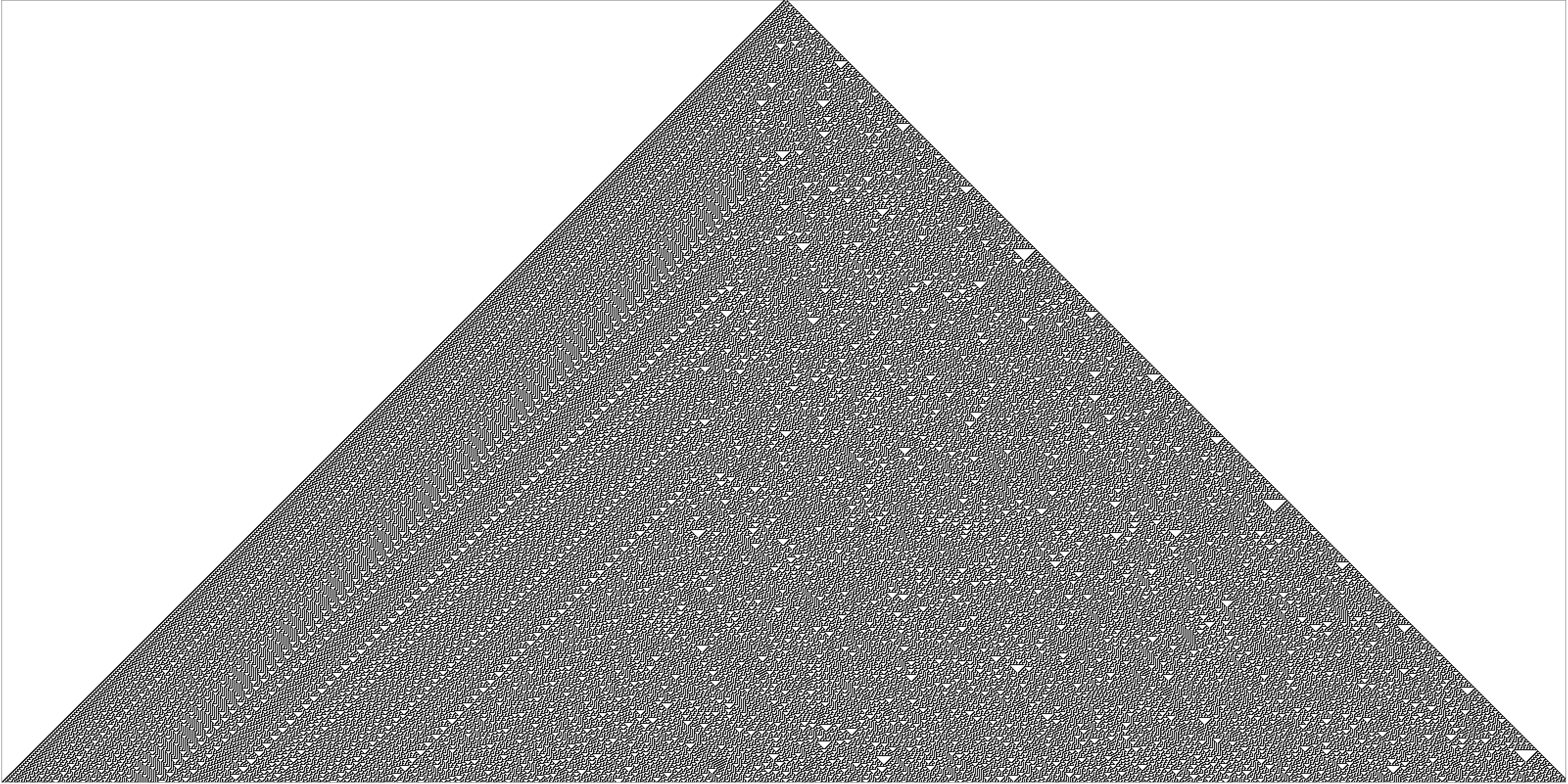
On the left side, we clearly see some repetition and some homogeneity, though things aren’t quite as predictable as they were for rule \(110\). But on the right side we see chaotic behavior. The boundary between these two regions is not a vertical line, but instead seems to drift back and forth across the center of the triangle.

There’s a family of questions related to rule \(30\), which I’ll only paraphrase here. First, a definition. We’ll use \(\mathbb{Z}\) to index the cells on which we’ll run this automaton, and in the initial configuration we set cell \(0\) to be black while the rest of the cells are white. Define a sequence \(\{c_{n}\}\) by

\[c_n = \begin{cases} 1 & \text{if cell}~0~\text{is black after}~n~\text{iterations} \\ 0 & \text{if cell}~0~\text{is white after}~n~\text{iterations}\end{cases}\]

In other words, \(\{c_n\}\) is a sequence of \(0\)s and \(1\)s corresponding to the middle column of the output of rule \(30\), as seen here.

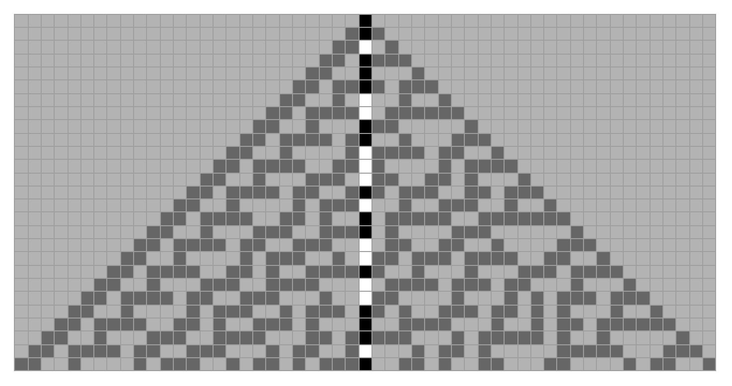
So the sequence \(\{c_n\}\) begins as follows

\[1,1,0,1,1,1,0,0,1,1,0,0,0,1,0,1,1,0,0,1,0,0,1,1,1,0,1,\ldots\]

and you can read more about this sequence at the relevant OEIS entry. Studying the behavior of rule \(30\) has led to several hard questions. Informally, they are:

1. Is \(\{c_n\}\) eventually periodic?
2. Does \(\{c_n\}\) have the same number of \(0\)s and \(1s\) (asymptotically)?
3. How hard is it to compute \(c_n\)?

These questions, when stated more rigorously, comprise the Rule 30 Prize Questions, and you can read a lot of interesting background, motivations, partial results, and generalizations here. It’s worth noting that this is not the first automaton-related question for which Wolfram Research has offered prize money. They previously offered prize money for a definitive answer to a question about a \(2\)-state, \(3\)-color turing machine question, and they later ended up accepting a solution.

Since this post came from a talk aimed at undergraduates, I have essentially nothing further to say about these questions. Instead, the key takeaway from this discussion might be summarized as follows: Simple rules can lead to complicated behavior and deep unanswered questions.

But I want to breeze past these deep unanswered questions to talk about some other \(1\)-dimensional cellular automata that are natural generalization of the elementary cellular automata discussed above.

Multi-state generalizations

The first generalization you might think of is increasing the number of states. The rules above were visualized by using black and white squares to represent the two possible states of a cell. So increasing the number of states is easy to represent visually. We’ll just use more colors.

For a nice example, let’s consider a cellular automaton that has three states, represented by white, blue and yellow. Here’s a visualization of the rule we’ll follow.

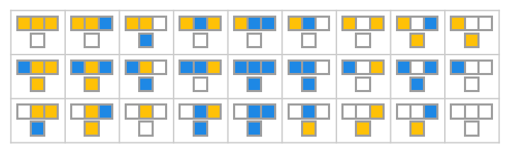
As you can see, we had to make \(27\) choices in order to specify a rule, and for each choice we have three options. Three-color cellular automata like this one are specified not by a binary string of length \(8\) but by a ternary string of length \(27\). This one is

\[001000022221011010120112220_3\]

which is the decimal integer \(285889819218\) if you’re keeping track. Mathematica knows all about these generalized \(1\)-dimensional cellular automata, so working with them and producing visualizations is as easy as ever. All you need is the rule number and the number of colors. We can work with this one in particular with CellularAutomaton[{285889819218, 3}]. I chose this rule in particular not only because it has an interesting mix of ordered and disordered behavior, but also because it is highly sensitive to initial conditions in an interesting way.

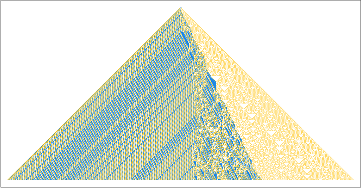
Let’s start by looking at what happens after \(400\) steps starting from a single blue square on a white background.

ArrayPlot[CellularAutomaton[{idx, 3},{{1}, 0},400], 
          ColorRules -> {1 -> RGBColor["#1E88E5"],
                         2 -> RGBColor["#FFC107"]}]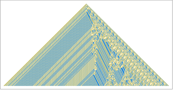

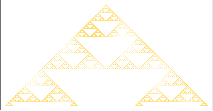
And if you push past \(400\) steps a semi-pattern becomes more apparent. There’s somewhat ordered striping to the left, highly ordered striping on the right, but a disordered region near the middle. However, if we instead started with a single yellow square on a white background, we get much simpler Sierpinski triangle-like behavior.

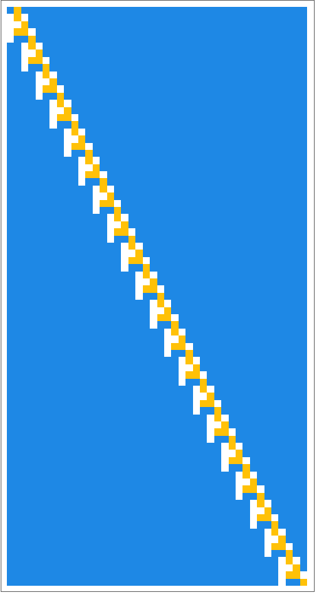
But you could also start with a single yellow square on a blue background, which gives you something even simpler. Borrowing terminology from Conway’s game of life, you might call this a “glider”. A recurrent pattren moving to the right forever.

Finally, we can start with something a bit more complicated. Let’s try this initial configuration on a white background.

We end up with the following.

This has some features in common with the first image above, but now the right side of the triangle is a region without blue squares, but where the white and yellow squares are exhibiting what you might call rule \(30\)-like chaotic behavior.

More complex rules

In all the one-dimensional cellular automata we’ve talked about so far, each cell is updated based on its own state and the states of its two neighbors. We’ll get a more general class of rules if we allow each cell’s behavior to be determined by itself and it’s four nearest neighbors. Here’s an example of such a rule.

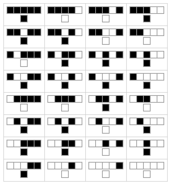
Once again, Mathematica knows about these. In fact it’s maybe worth pointing out here that the Mathematica documentation for CellularAutomata gives details on how to specify and work with a variety of different generalizations. For this one in particular, the specification looks a little different, but once we have it we can work with this rule as easily as the preceeding rules.

CellularAutomaton[<|"RuleNumber" -> 2625580504, "Range" -> 2|>]

As usual we start with a single black cell and watch what happens

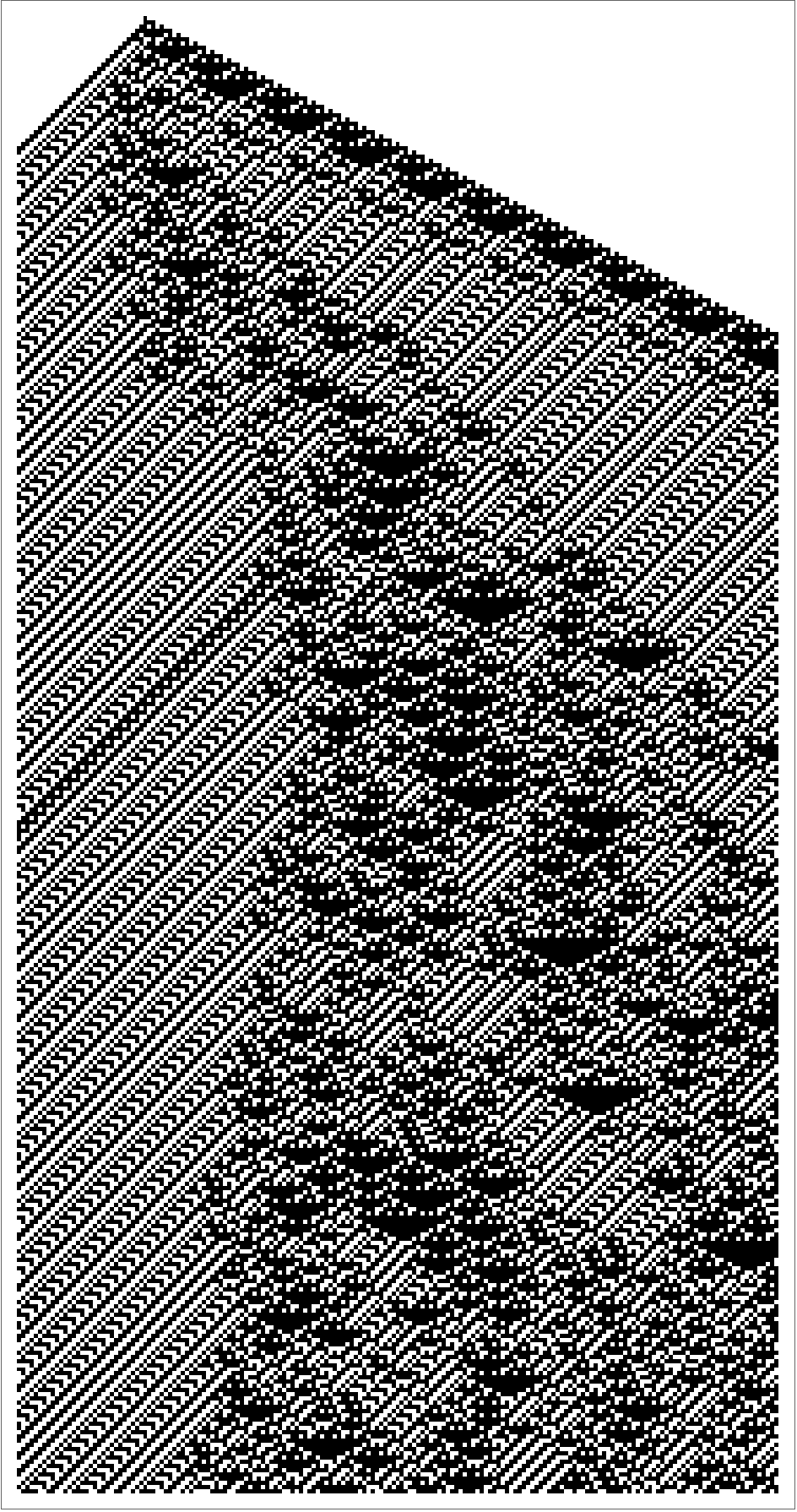
As in the earlier examples, we see three visually-distinct regions. A highly-structured region on the right, a quite structured but not repetitive region to the left, and a disordered and chaotic region in the middle.

It’s not a coincidence that many of the automata in my talk and in this post have this feature. I have deliberately chosen them this way, since this makes for the most visually appealing examples. But you should not expect every automaton you look at to behave like this. There’s more that can happen.

Classes of behavior

In fact, there is a heuristic classification scheme for automata, grouping them into four classes depending on their behavior. You can find this classifcation scheme, along with much more discussion of automata and some cool pictures, in Stephen Wolfram’s book “A New Kind of Science”. For the particular discussion of classifying automata according to their behavior, see here in chapter 6. The four categories of automata behavior are (and I’m paraphrasing here):

1. Almost immediately trivial.
2. Eventually predictable.
3. Chaos.
4. Structured chaos.

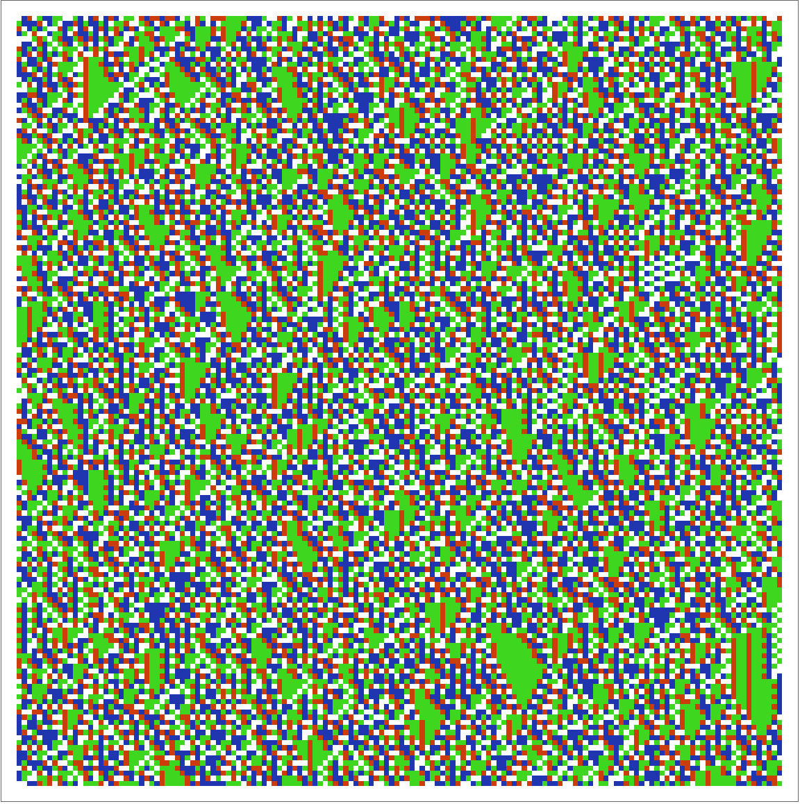
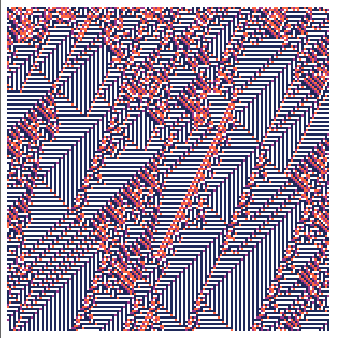
These categories are not rigorously defined, but after looking at a lot of examples of cellular automata you’ll start to notice that this system of classifications is a good and sensible one. I’ll wrap up this post with a representative example of each class, chosen from among the range \(1\) cellular automata with \(4\) states. In a slight variation on the above, these automata take place on a finite and circular array of \(150\) with wrapping, and with a random initial configuration, but the ideas are the same.

Class 1 automata quickly settle into a stable and homogenous state.

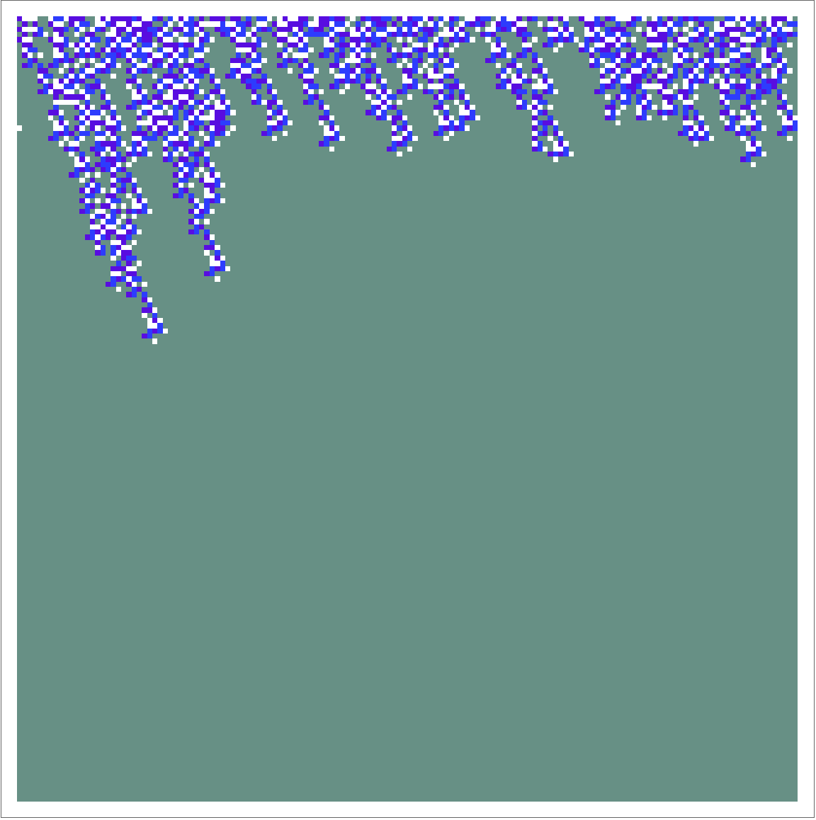Class 2 automata may have some stable structures or gliders, but they eventually fall into a state that’s stable, periodic or otherwise predictable.

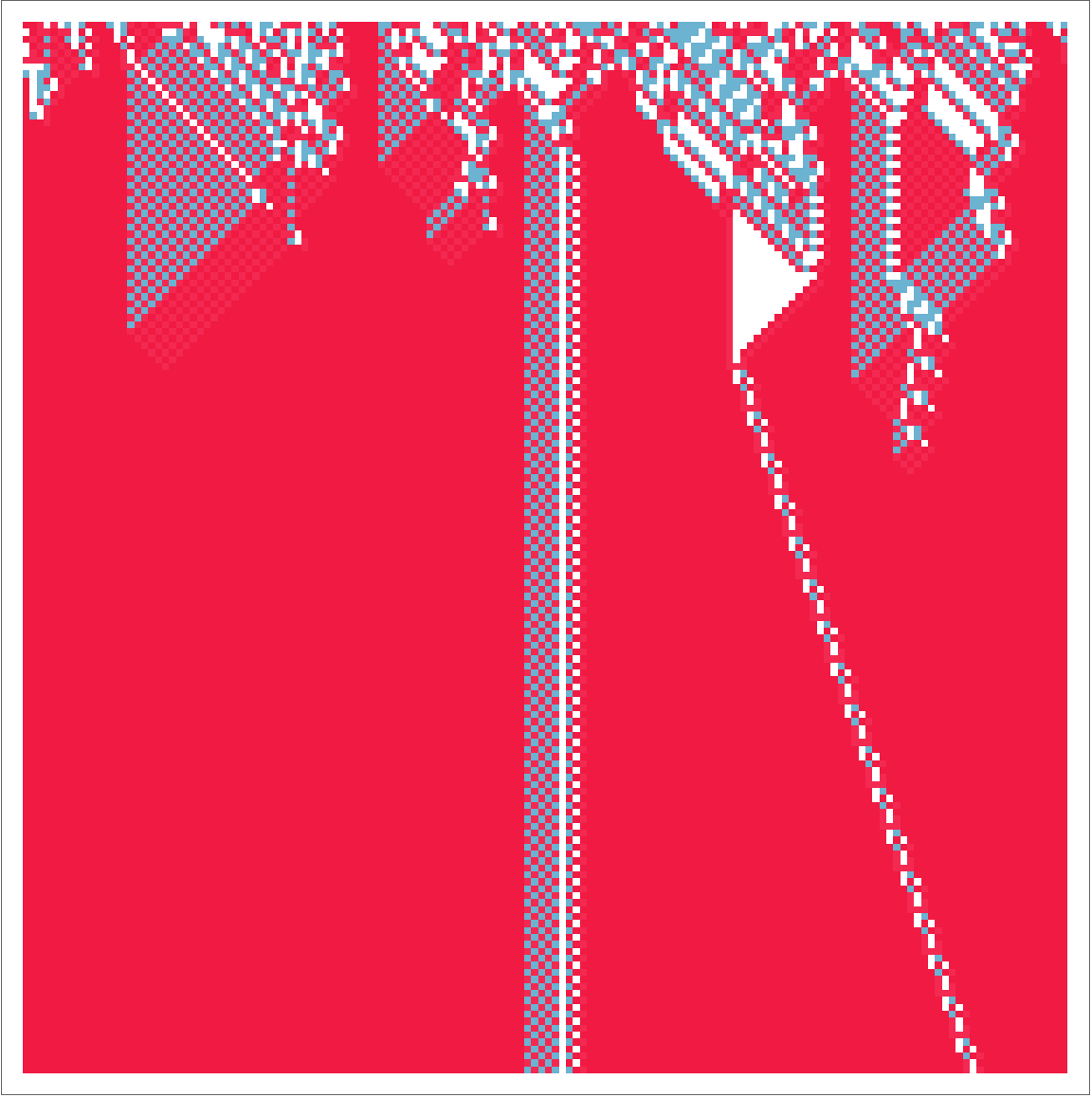
Class 3 automata are chaotic. They may exhibit small recurrent motifs or a distinctive texture, but the overall behavior is unpredictable and disordered.

Class 4 automata show a mix of chaos and structure. There may be large recurrent motifs or large textured regions, or entire regions of repetition and predictability. But no global structure or stability.

The second half of my talk covered Langton’s ant. I intend to summarize that part of the talk in a follow up post.