
Cellular automata and Langton's ant - part II
29 Mar 2020This is the second in a series of posts summarizing a talk I gave for the Undergraduate Math Club at the University of Kentucky. The first post covered one-dimensional cellular automata. In this post I’ll cover the second half of the talk, Langton’s ant and its generalizations.
Langton’s ant
Langton’s ant was first described in this paper, where it was given as an instance of a vant, short for “virtual ant”. That terminology doesn’t seem to have caught on, and this object and its generalizations are now referred to as Langton’s ants or turmites, as we’ll see below. The original motivation seems to have been quite cross-disciplinary, at the intersection of cellular automata and biochemistry, and possibly evolutionary biology. The extent to which this direction of research has borne fruit is not clear to me. But Langton’s ant and turmites are also interesting from the point of view of abstract computer science and mathematics.
The original Langton’s ant refers to the following automaton. Start with an infinite \(2\)-dimensional grid of squares. Each square can be either white or black, but initially all squares are white.
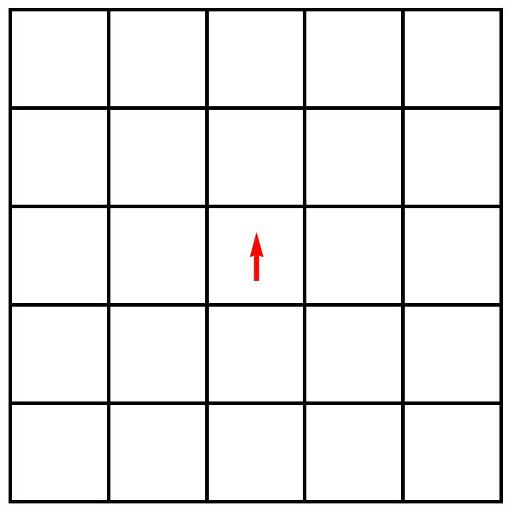
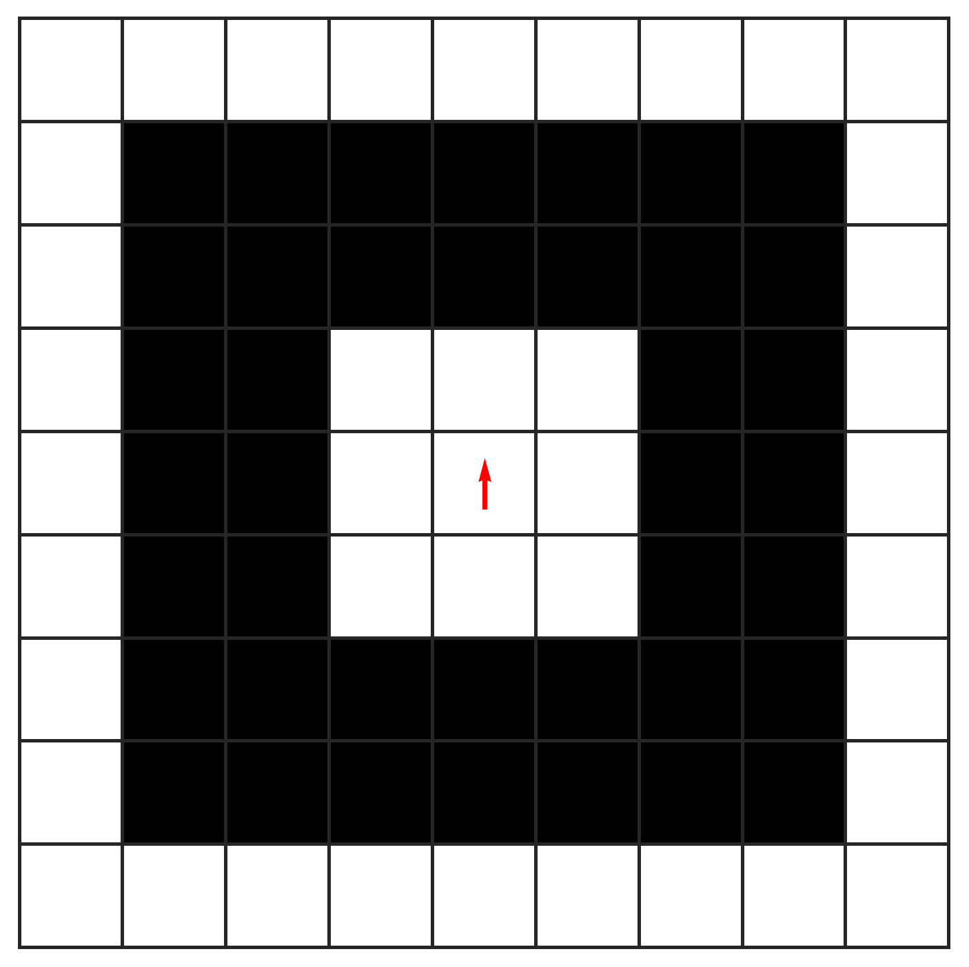
On this grid of squares there’s an ant. The ant can be located in any of the squares, and it can be facing in any of the four cardinal directions. Let’s say initially it’s facing north. Using a red arrow to represent the ant’s location and direction, here’s the initial state of our automaton.
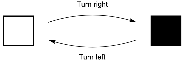
The ant’s behavior is determined by two simple rules:
- If the ant is on a white square, it turns \(90^{\circ}\) to the right, toggles the square to black, then steps one square forward in the direction it’s facing.
- If the ant is on a black square, it turns \(90^{\circ}\) to the left, toggles the square to white, then steps one square forward in the direction it’s facing.
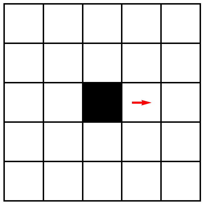
Let’s apply this rule to the initial configuration shown above. The ant is on a white square. So it will turn so that it’s facing east. Then it will toggle its square to black, then it will step one square to the east. After that, we’ll be in this configuration.
You can run this process by hand if you want, though it’s easier to automate it. Here’s a small animation that shows the behavior of this ant as it takes its first \(200\) steps.
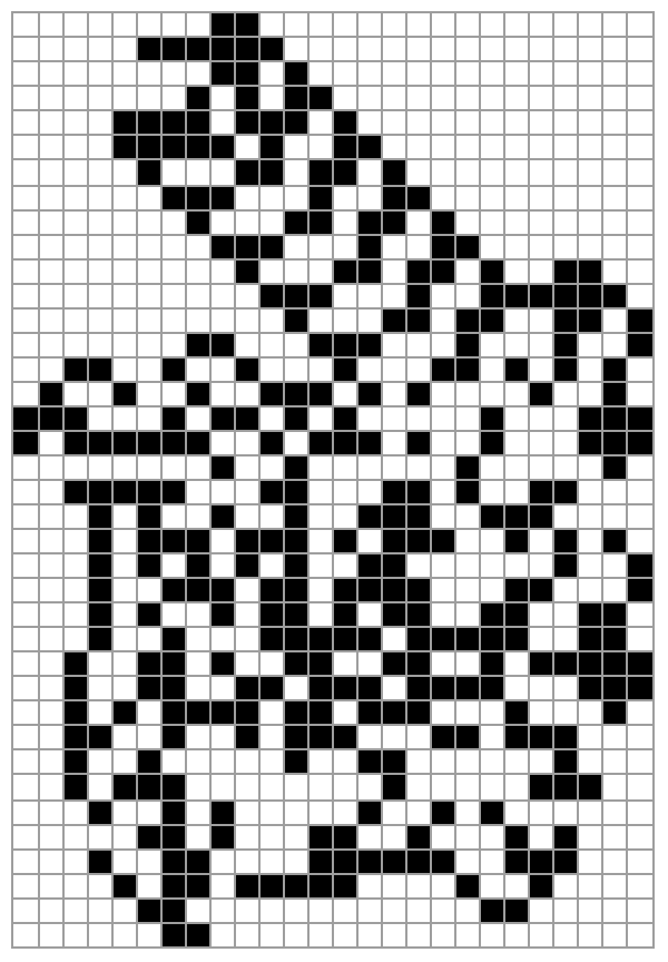
The reasonable question at this point is: what happens in the long run? Well, let’s just run it and see. Here is the configuration of black squares in the grid after \(200\) steps:
After \(1{,}000\) steps:
And here’s how things look after \(10{,}000\) steps
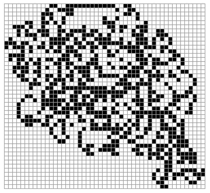
At this point it looks like a giant chaotic mess. But if we push any further, we start to see something interesting. Here’s the state of things after after \(11{,}500\) steps.
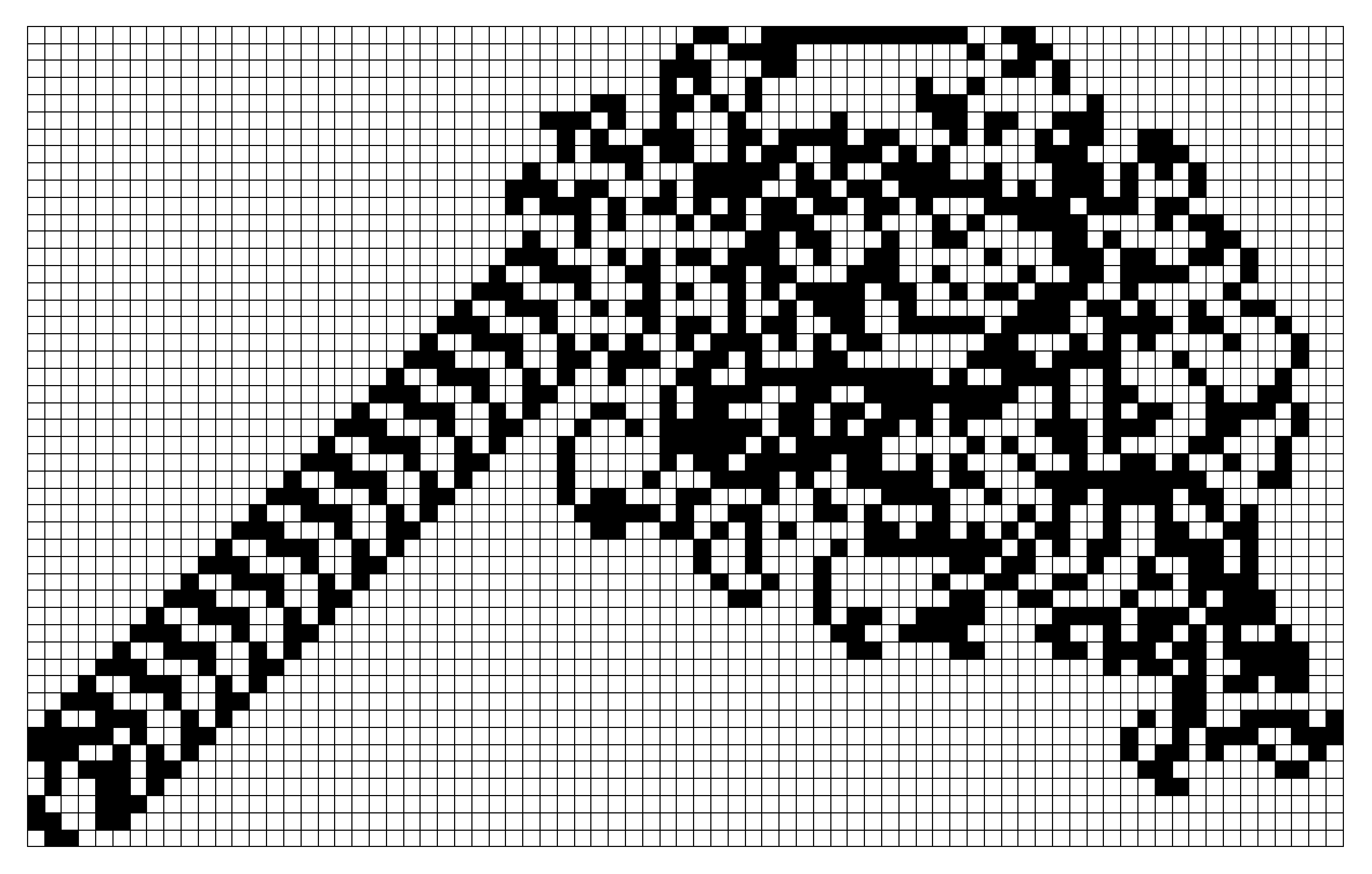
It turns out that beginning at step \(9{,}978\), the ant starts to repeat the same sequence of \(104\) moves over and over again, and this repetitive behavior results in the structure you see here, often referred to as a “highway”. You should maybe think of this as the same kind of phenomenon described in the last post: a very simple rule leading to a mix of two things: some disorder and chaos, but also some order and structure.
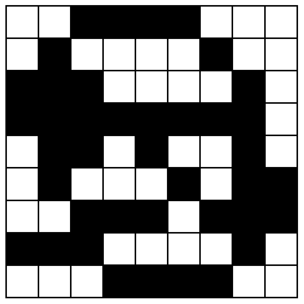
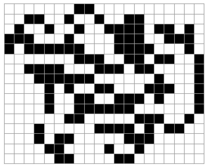
One way you might try to study the behavior of Langton’s ant is to vary the initial configuration of the grid of cells. It’s straightfoward to see that if you start on an infinite grid of black squares, the ant produces a mirrored version of the pattern above. But you could instead run the ant on a grid with a more complicated initial configuration of black and white squares. For example, you could start from this initial configuration:
It turns out you’ll still get a chaotic region followed by that same \(104\)-step highway. This time it takes about \(3{,}000\) steps for the ant to start its highway.
Doing a lot of experimentation might lead you to make the following conjectures. If you run Langton’s ant on an initial configuration with finitely many black squares:
- The ant will eventually form a highway.
- The highway will be (a rotation or reflection of) the same \(104\)-step highway.
As far as I know, these conjectures are wide open. It’s pretty straightforward to prove that the set of squares visited by the ant is unbounded. But that’s really far from addressing either of the conjectures above. Why can’t the ant just form a chaotic region without ever falling into its highway behavior? And why can’t there be another, more complicated (or simpler) highway that the ant builds when we set it up with just the right initial configuration?
These questions are likely extremely difficult and I don’t even know how to begin to approach them. So instead, let’s talk about generalizations of Langton’s ant.
Ants with additional colors
One of the most well-known generalizations of Langton’s ant is ant-like automata that use more than two colors.
Suppose that instead of just white and black, the ant knows about \(n\) colors, called \(c_1, \ldots, c_n\). The squares of the grid are initially all colored \(c_1\), and when the ant is on a square with color \(c_i\), it turns right or left depending on \(i\), then it updates the square’s color to \(c_{i+1}\) (with \(c_n\) wrapping back around to \(c_1\)). With this perspective, the original Langton’s ant can be represented with this labeled \(2\)-cycle describing the ant’s behavior on a white or black square.
But a four-color ant would have a rule represented by a labeled \(4\)-cycle, an example of which is shown here.
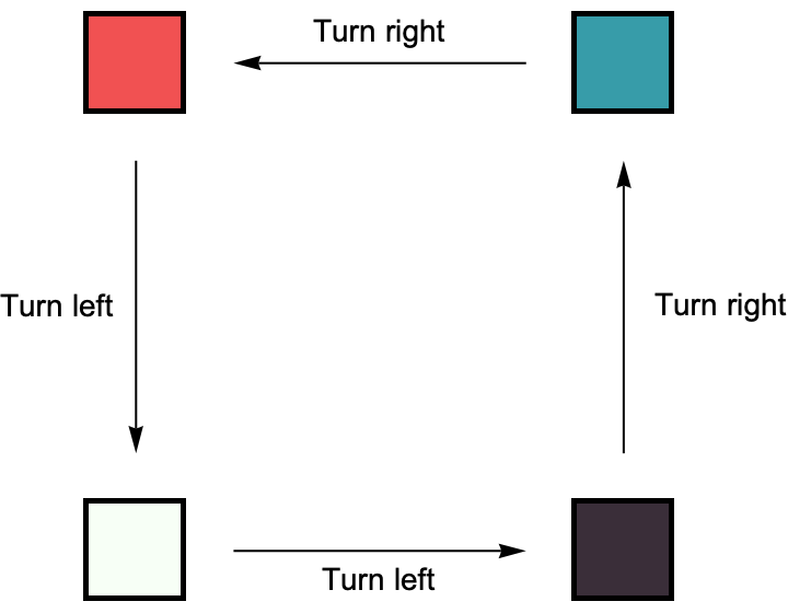
For an ant with \(n\) colors, it’s behavior is completely determined by whether it turns right or left on each of the \(n\) colors. So instead of using these cumbersome directed graph representations, we can specify one of these generalized ants just using a string of R and L characters representing these turns. in this notation, the original Langton’s ant is written RL, while the four color ant above would be represented by LRRL, assuming that the bottom left color is its initial color.
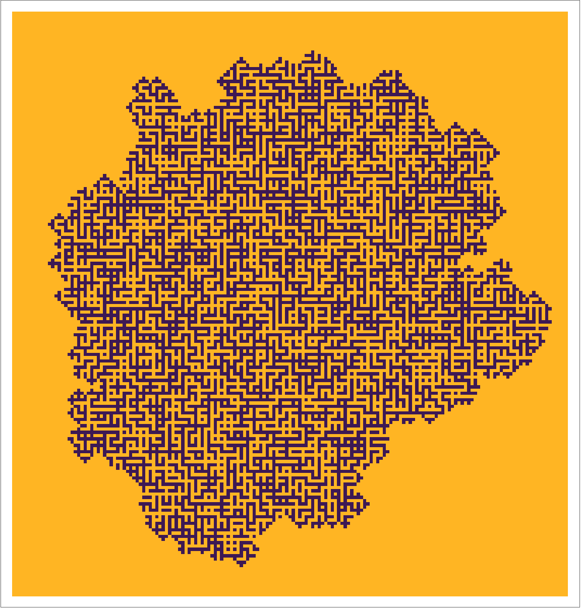
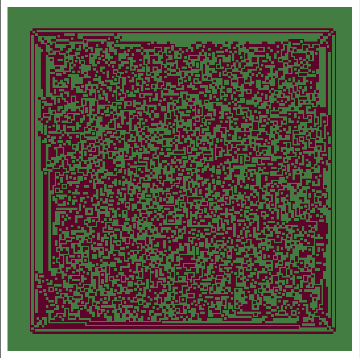
The behavior of this LRRL ant is visually quite different from the RL Langton’s ant. After \(20{,}000\) steps, the \(4\)-color grid looks like this

Then after \(200{,}000\) steps:
After \(2{,}000{,}000\) steps:
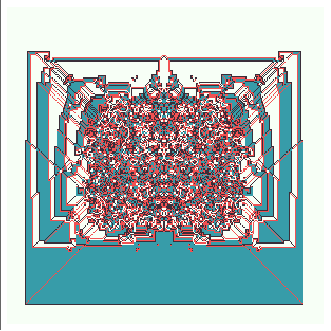
And finally after nearly \(20{,}000{,}000\) steps:
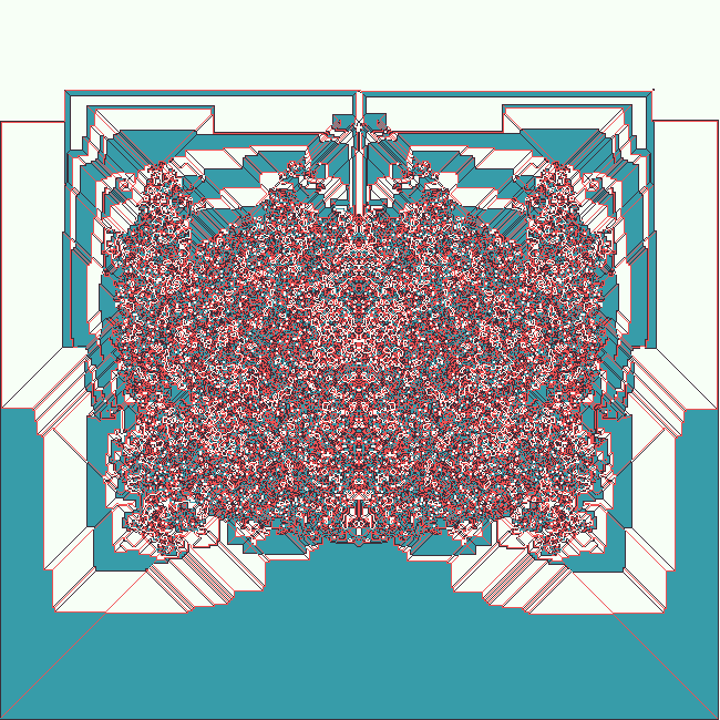
We still see a chaotic region in the middle and some uniform structurs around the edges, so you could plausibly call this a class 4 automaton.
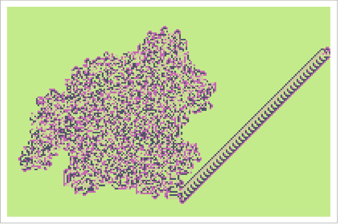
Many of these multi-colored ants still produce highways, like LLRL.
And LLRLRRLL.
And RRLRLLRRRRLL.
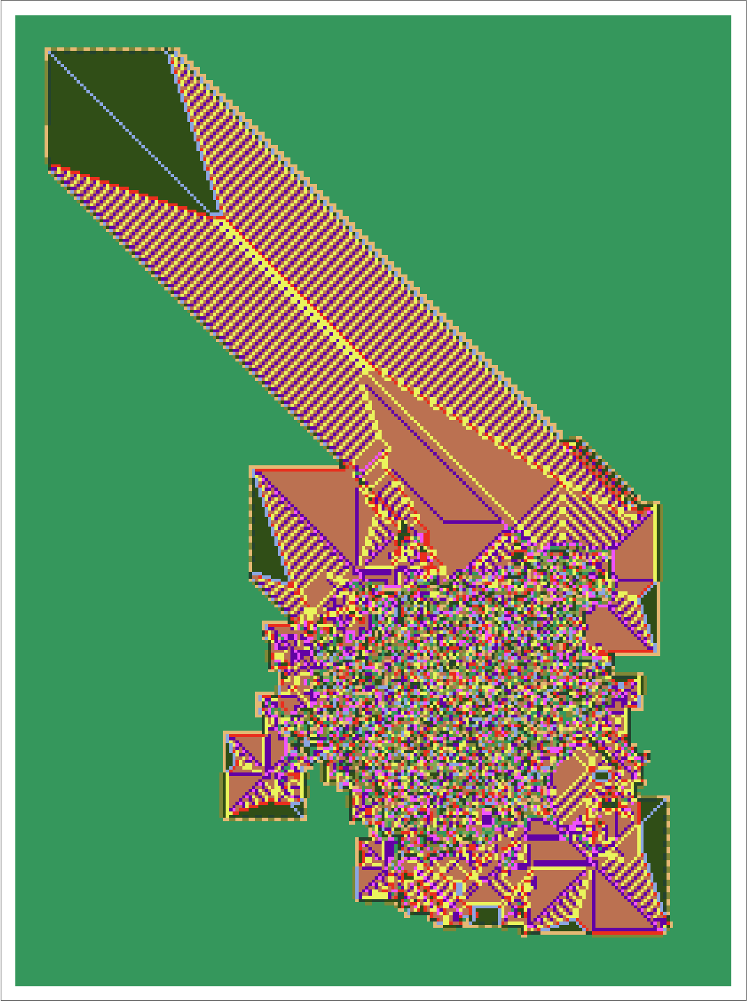
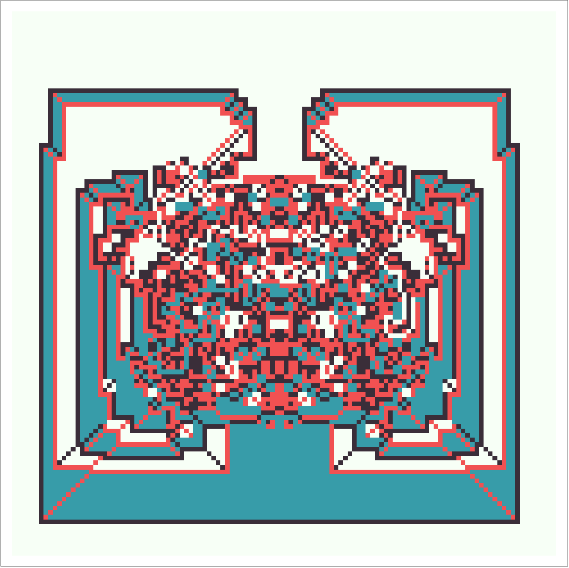
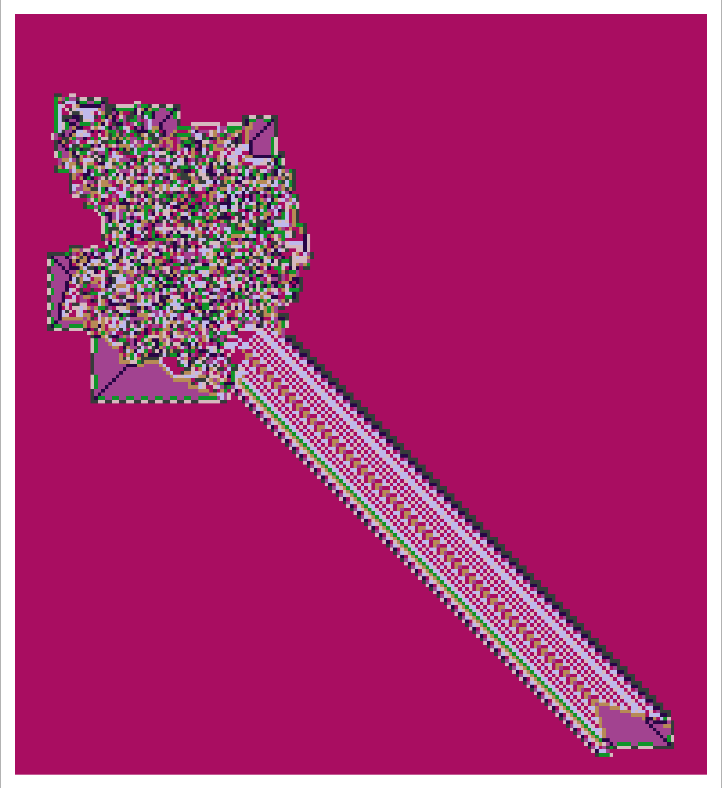
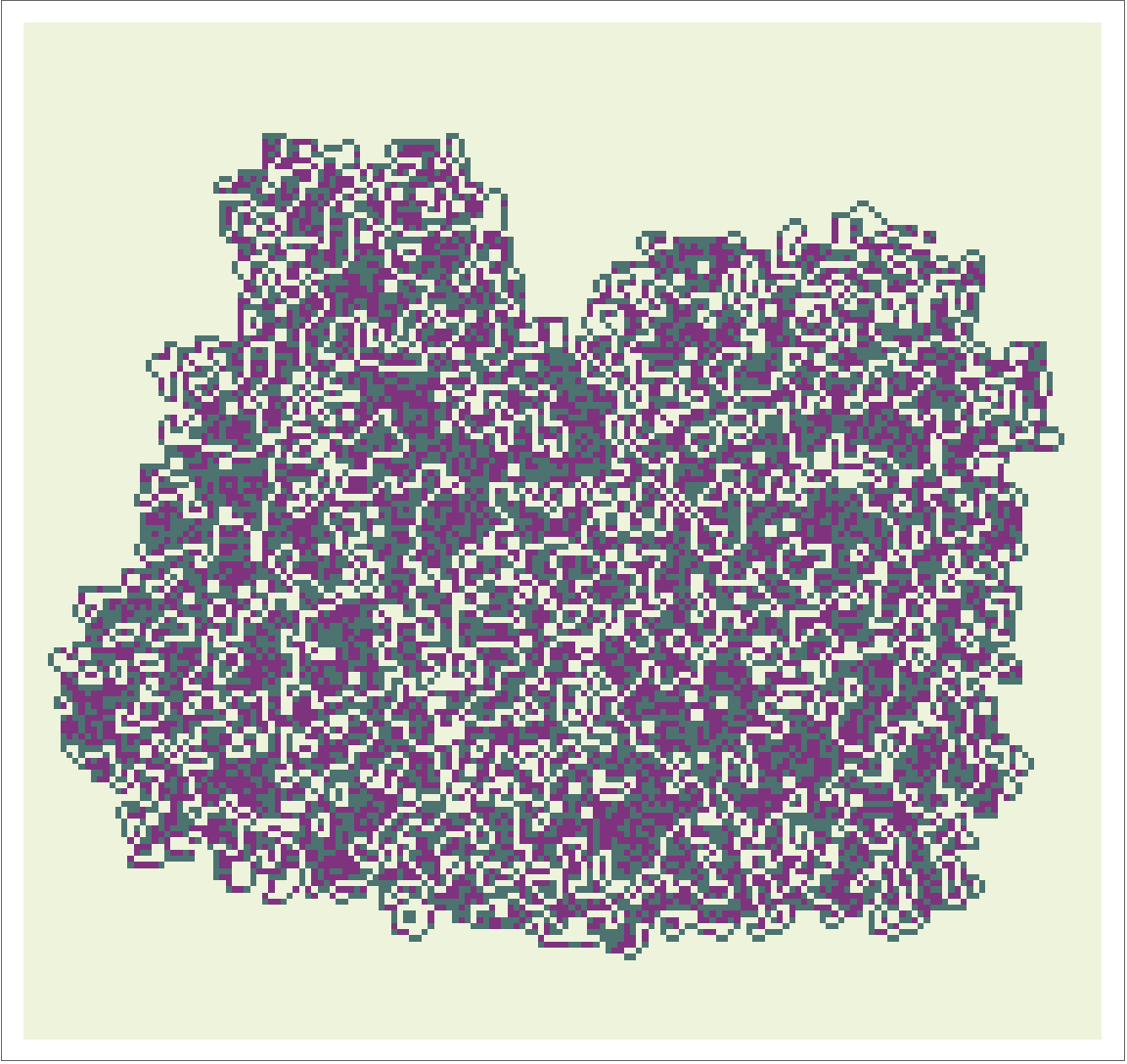
Though others, like LRRL above, produce an expanding structured region with a blotch of disorder in the middle. Another example of this behavior comes from RRLRRRLLLLLL.
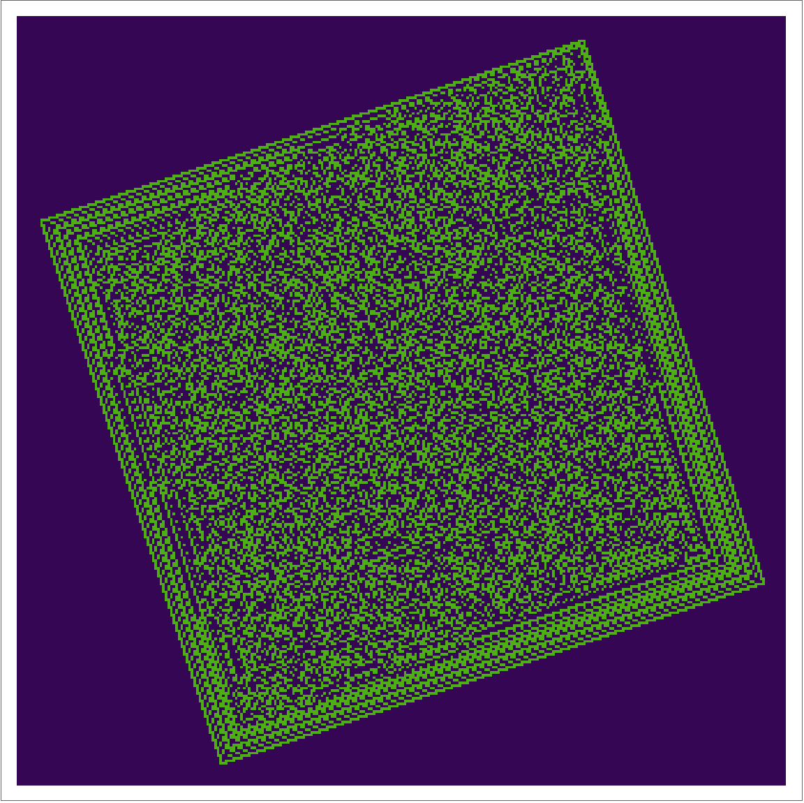
The set of cells visited by the ant RRLL after n steps looks like it’s bounded by a cardiod-like shape that depends on \(n\). Here’s RRLL after \(10{,}000{,}000\) steps.
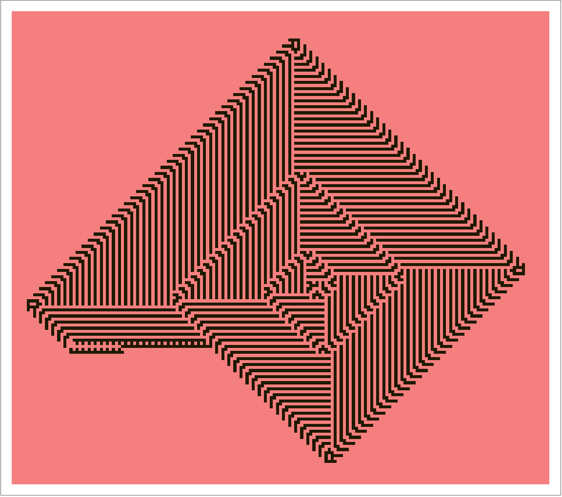
And some of these ants, like LRL, give no indication of any global structure nor do they seem to form a highway. As far as I know LRL has not yet been observed to form a highway, but empirical evidence is not a proof. Maybe we simply haven’t let it run long enough. I’d guess that proving any of of these observational conjectures is roughly as difficult to the original Langton’s ant problem. Here’s LRL after \(2{,}000{,}000\) steps.
Further generalizations
There are many further generalizations of Langton’s ant beyond just increasing the number of colors. You often see ants with more moves than just L and R. Sometimes there’s a U move for a \(180^{\circ}\) turn and an N move for a \(0^{\circ}\) turn.
You also see generalizations to different grids of cells, like a grid of hexagons or equilateral triangles, or to a \(3\)-dimensional grid of cubes.
At some point I’d like to think about the following generalization. Replace the data of the ant’s cardinal direction with an arbitrary vector \(v\) in \(\mathbb{Z}^2\), and replace “turning” \(v\) with multiplication by a matrix in \(\operatorname{GL}(2,\mathbb{Z})\). More concretely, in the \(n\) color case, instead of a length \(n\) string of Ls and Rs, you choose a length \(n\) string of matrices \[\left\{m_i \in \operatorname{GL}(2,\mathbb{Z})\right | 1 \leqslant i \leqslant n\}\] so that on color \(c_i\) the ant’s direction vector \(v\) is updated to \(g_i \cdot v\). But that’s a project for a later date.
Turmites: ants with internal states.
I’ll close with one more generalization of Langton’s ant. This last object is a cellular automaton called a turmite. This is a simultaneous generalization of Langton’s ant and of Turing machines, though in a sense which can be made precise, turmites are not any more general than ordinary Turing machines.
A turmite is a \(2\)-dimensional cellular automaton, like Langton’s ant. It exists on a an infinite grid of squares, each of which can be any of \(n\) colors. But a turmite also has a set of \(m\) internal states. The turmite’s behavior on a square is determined not only by the color of that square but also by which internal state the turmite is in at that time. When the turmite updates a square’s color and steps onto a new square, it also deterministically updates its internal state.
More formally, a turmite has \(m\) internal states \(S=\{s_1, \ldots, s_m\}\), and the squares in its grid can be any of the \(n\) colors from the set \(C=\{c_1, \ldots, c_n\}\). Initially, the turmite is located on a grid of squares all colored \(c_1\), and it is pointing north. The turmite’s behavior on a given square is governed by three functions.
\[f_{\text{color}} :S \times C \to C\] \[f_{\text{state}} :S \times C \to S\] \[f_{\text{turn}} :S \times C \to \{0,1,2,3\}\]
Here’s how it works. Suppose the turmite’s internal state is \(s\) and it’s standing on a square with color \(c\). In this case, the turmite updates the square’s color to \(f_{\text{color}}(s,c)\), updates its internal state to \(f_{\text{state}}(s,c)\), and turns \(90^{\circ}\) to the left \(f_{\text{turn}}(s,c)\) times. We can represent these three functions as \(m \times n\) matrices over \(C\), \(S\) and \(\{0,1,2,3\}\) respectively. For brevity we will identify \(C\) and \(S\) with their sets of indices, which means all of our matrix entries will be integers.
With this notation, the original Langton’s ant can be represented as a turmite.
\[f_{\text{color}} = \begin{pmatrix} 2 & 1 \end{pmatrix}, f_{\text{state}} = \begin{pmatrix} 1 & 1 \end{pmatrix}, f_{\text{turn}} = \begin{pmatrix} 1 & 3 \end{pmatrix},\]
A \(12\)-color ant like RRLRLLRRRRLL can also be written as a turmite.
\[f_{\text{color}} = \begin{pmatrix} 2&3&4&5&6&7&8&9&10&11&12&1 \end{pmatrix}\] \[f_{\text{state}} = \begin{pmatrix} 1&1&1&1&1&1&1&1&1&1&1&1 \end{pmatrix}\] \[f_{\text{turn}} = \begin{pmatrix} 3&3&1&3&1&1&3&3&3&3&1&1 \end{pmatrix}.\]
Of course, the interesting examples come from turmites that actually have more than one internal state. Here are a few, with visualizations.
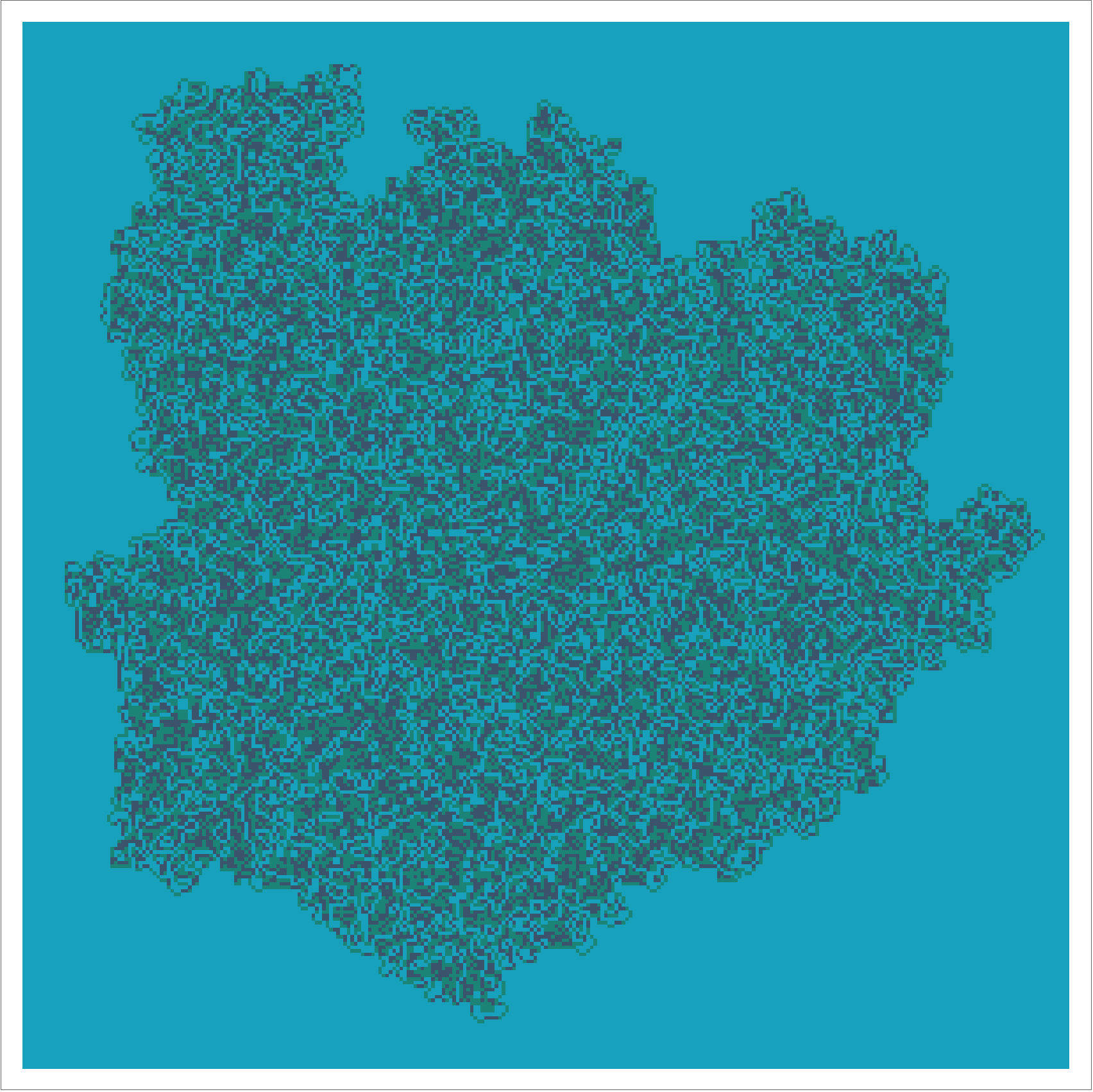
You can find some interesting textured regions with no apparent highway.
\[f_{\text{color}} = \begin{pmatrix} 2 & 2 \\ 2 & 1 \end{pmatrix}, f_{\text{state}} = \begin{pmatrix} 1 & 2 \\ 1 & 1 \end{pmatrix}, f_{\text{turn}} = \begin{pmatrix} 2 & 1 \\ 2 & 0 \end{pmatrix},\]
\[f_{\text{color}} = \begin{pmatrix} 2 & 3 & 1\\ 2 & 3 & 1 \end{pmatrix}, f_{\text{state}} = \begin{pmatrix} 1 & 1 & 2 \\ 2 & 2 & 2 \end{pmatrix}, f_{\text{turn}} = \begin{pmatrix} 3 & 3 & 3 \\ 3 & 1 & 3 \end{pmatrix},\]
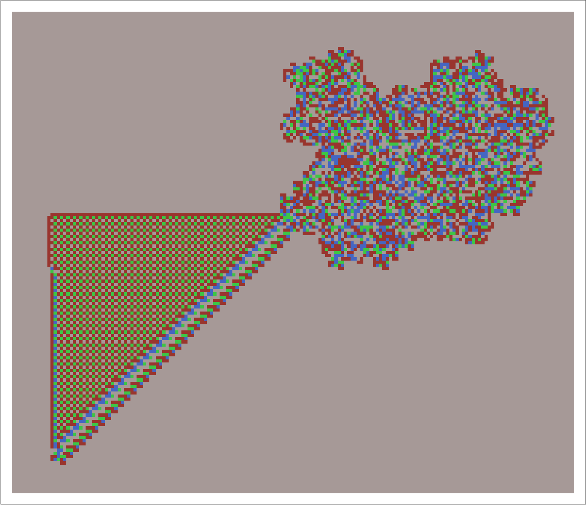
You also see turmites that form highways after a period of chaotic behavior, like this one.
\[f_{\text{color}} = \begin{pmatrix} 2 & 3 & 4 & 1\\ 2 & 4 & 2 & 1 \end{pmatrix}, f_{\text{state}} = \begin{pmatrix} 2&2&2&2 \\ 2&1&2&1 \end{pmatrix}, f_{\text{turn}} = \begin{pmatrix} 3&1&3&3 \\ 3&1&3&1 \end{pmatrix},\]
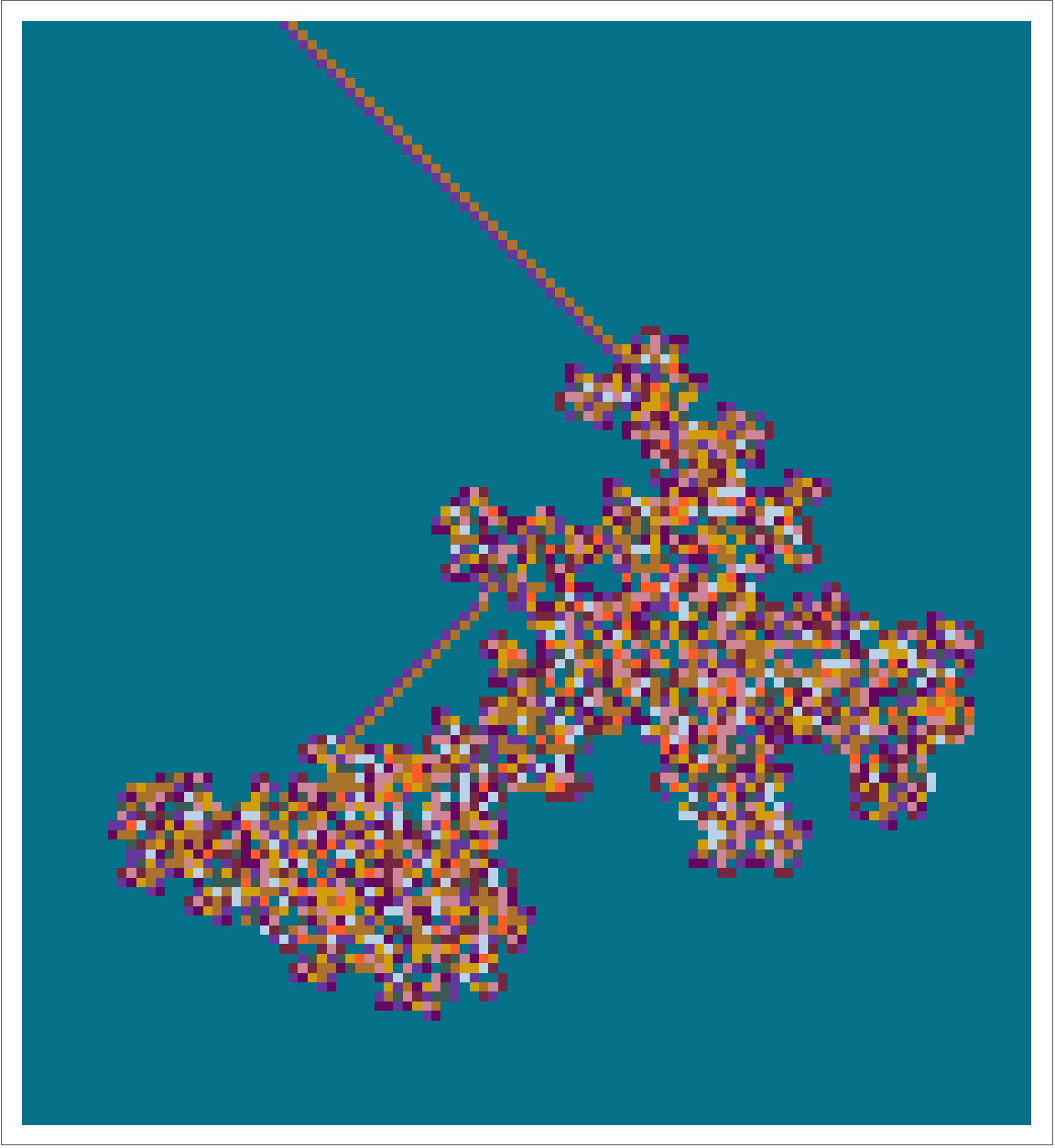
Here’s a \(10\)-color, \(10\)-state turmite, found by a random search, which eventually finds its way to producing a very simple highway, but the highway leads it back into its own chaotic region. It then produces a bit more chaos before eventually starting the simple highway again, this time for good.
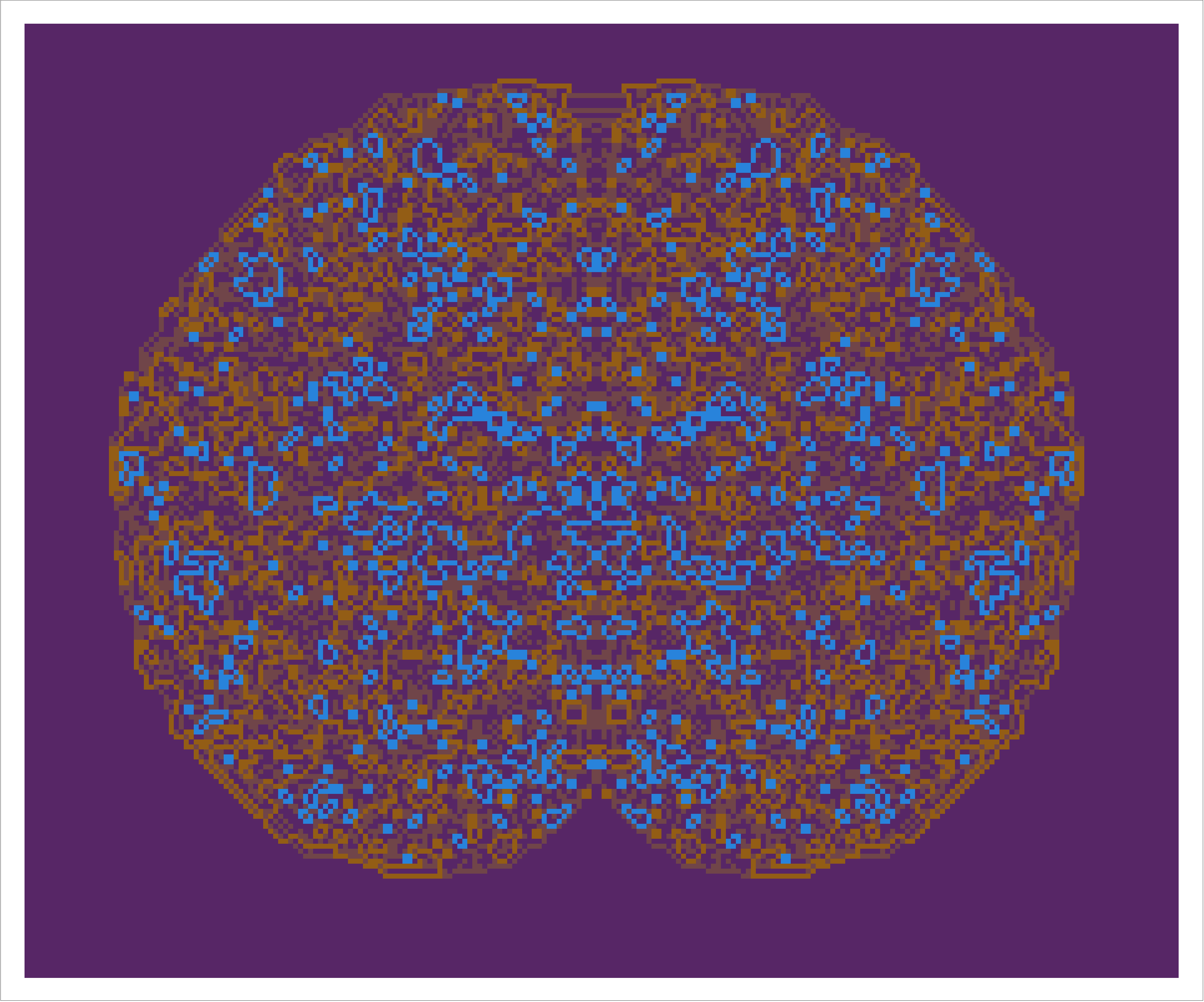
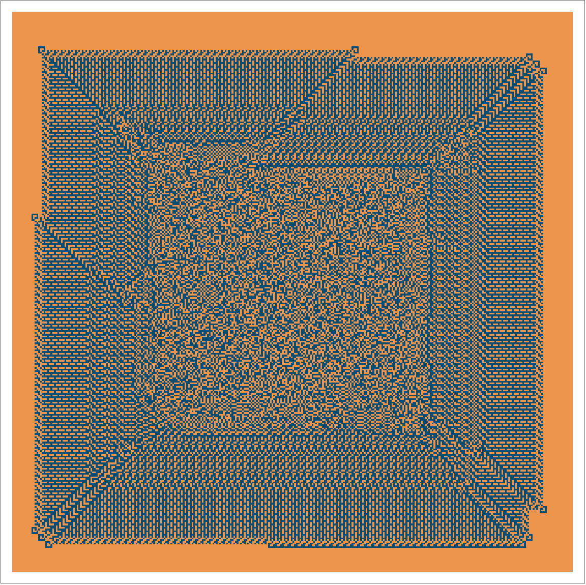
Translating one of the examples from Wikipedia into our own notation and pushing it a little farther, we run \(20{,}000{,}000\) steps of this turmite below.
\[f_{\text{color}} = \begin{pmatrix} 2 & 2 \\ 1 & 1 \end{pmatrix}, f_{\text{state}} = \begin{pmatrix} 1 & 2 \\ 1 & 2 \end{pmatrix}, f_{\text{turn}} = \begin{pmatrix} 1 & 3 \\ 3 & 1 \end{pmatrix},\]
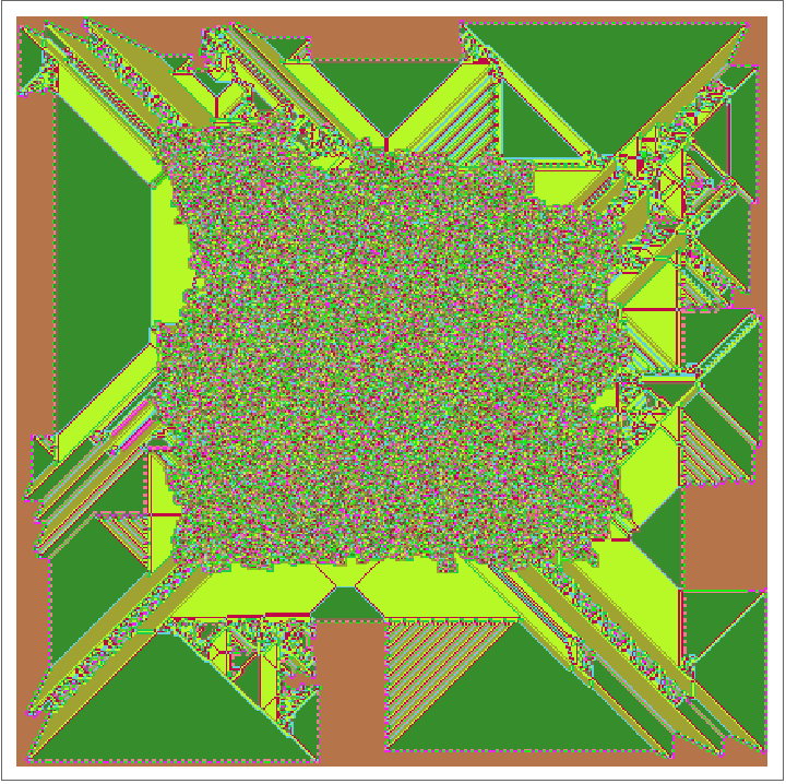
There are other turmites with similar behavior, forming a square with an irregular texture, like this one.
\[f_{\text{color}} = \begin{pmatrix} 2 & 2 \\ 2 & 1 \end{pmatrix}, f_{\text{state}} = \begin{pmatrix} 2 & 2 \\ 1 & 2 \end{pmatrix}, f_{\text{turn}} = \begin{pmatrix} 3 & 3 \\ 0 & 1 \end{pmatrix},\]
Or this one.
\[f_{\text{color}} = \begin{pmatrix} 2 & 2 \\ 2 & 1 \end{pmatrix}, f_{\text{state}} = \begin{pmatrix} 2 & 2 \\ 2 & 1 \end{pmatrix}, f_{\text{turn}} = \begin{pmatrix} 0 & 0 \\ 1 & 0 \end{pmatrix},\]
But you also sometimes see highly regular behavior, like this turmite that immediately produces a regular spiral.
\[f_{\text{color}} = \begin{pmatrix} 1 & 1 \\ 2 & 1 \end{pmatrix}, f_{\text{state}} = \begin{pmatrix} 2 & 1 \\ 2 & 1 \end{pmatrix}, f_{\text{turn}} = \begin{pmatrix} 1 & 3 \\ 3 & 1 \end{pmatrix},\]
Even restricting your attention to the \(2\)-color, \(2\)-state turmites, there’s a lot of variety. But they do still seem stratified into the four informal classes of automata discussed earlier.
Langton’s ant animations and videos.
All of the images and animations in this series of posts were made by me, using Mathematica.
But I ended my talk with some videos I had made showing the behavior of multi-colored generalized ants. I have not reproduced them here because they weren’t entirely my own work. Those videos were produced using this phenomenal piece of software. The author of that software, Ryan Wick, used it to make this video, which was what motivated me to put together this talk and to write these posts in the first place.
For some reason, ant animations that show hundreds of thousands of steps seemed pretty uninteresting to me. But animations showing hundreds of millions of steps compressed into just a few seconds seemed captivating and mysterious. Unfortunately, I could not squeeze enough performance out of Mathematica to make videos on the scale I wanted in a reasonable timeframe, while Ryan Wick’s animator produced them almost immediately.
The performance discrepancy between Mathematica and C++ in this case makes me want to try to write my own animation-maker that allows turmites or other generalizations, with a focus on performance. But that’s a project for another day.