N Fieldsteel

A Cayley table for SL(2,3)

This is a post about generating a Cayley table for the group \(\text{SL}(2,3)\) in a way that visualizes a maximal flag of normal subgroups, similar to my previous post about \(S_4\). I am going to take much of the underlying group theory for granted here, as the focus of this post is the idiomatic Mathematica code that makes generating this example so easy.

The group \(\text{SL}(2,3)\) is the set of all \(2 \times 2\) matrices with entries in \(\mathbb{Z}/3\mathbb{Z}\) with determinant equal to \(1\bmod{3}\). We give special names to four particular elements of this group.

\[e = \begin{bmatrix}1 & 0 \\ 0 & 1\end{bmatrix}, ~ i = \begin{bmatrix}1 & 1 \\ 1 & 2\end{bmatrix}, ~j = \begin{bmatrix}2 & 1 \\ 1 & 1\end{bmatrix}, ~ k = \begin{bmatrix}0 & 2 \\ 1 & 0\end{bmatrix}.\]

Or, in Mathematica:

e := {{1, 0}, {0, 1}};
i := {{1, 1}, {1, 2}};
j := {{2, 1}, {1, 1}};
k := {{0, 2}, {1, 0}};

As it turns out, the elements \(i,j\) and \(k\) generate a normal subgroup \(Q \trianglelefteq \text{SL}(2,3)\) with \(8\) elements, namely \({\pm e,\pm i, \pm j, \pm k}\). Up to isomorphism, this group \(Q\) is the group of Quaternions, and it is the maximal normal subgroup of \(\text{SL}(2,3)\). While every subgroup of \(Q\) is a normal subgroup of \(Q\), not every subgroup of \(Q\) is a normal subgroup of \(\text{SL}(2,3)\). But some of them are, and it turns out that the subgroup \(K = {\pm e}\) is the maximal subgroup of \(Q\) that is normal in \(\text{SL}(2,3)\). In Mathematica:

Q = {e, -e, i, -i, j, -j, k, -k};
K = {e, -e};

These lists are not ordered arbitrarily. In fact, we’ve ordered the elements so that \(Q\) is partitioned into the four left cosets of \(K\), namely \(K\), \(iK\), \(jK\) and \(kK\). Recall that for any group \(G\), any subgroup \(H \leqslant G\), and any choice of element \(g \in G\), the left coset of \(H\) represented by \(g\) is just the set

\[gH = \{g \cdot h ~|~ h \in H\},\]

which is easy enough to express in Mathematica, especially since our sets are actually lists and our group operation is matrix multiplication.

coset[g_, H_] := Table[g.h, {h, H}]

Now we (somewhat arbitrarily) choose coset representatives for the nontrivial cosets of \(Q\) in \(\text{SL}(2,3)\). For the element

\[r = \begin{bmatrix}1 & 2 \\ 0 & 1 \end{bmatrix},\]

the group \(\text{SL}(2,3)\) is a union of the three left cosets \(Q\), \(r Q\) and \(r^2 Q.\)

r = {{1, 2}, {0, 1}};
G = Join[Q, coset[r, Q], coset[r.r, Q]] // Mod[#, 3]&;

At this stage, \(G\) is a list of the elements of \(\text{SL}(2,3)\), but with a very carefully chosen ordering: the first eight, middle eight, and last eight elements are the cosets of \(Q\). And each of those three cosets is partitioned into left cosets of \(K\).

What we need next is not a natural group theoretic construction, but it will simplify the rest of our code: if G[[i]] represents the element at index i in our ordered group G, we want to know the index of G[[i]].G[[j]]. For example, G[[3]] is \(i\), while G[[9]] is \(r\). Their product is \(i\cdot r\), which is equal to \(r\cdot j\), which is G[[13]]. This fact (“third element times ninth element equals thirteenth element”) is really just the group operation for G, but where elements are referenced using their indices. This “group operation on indices” is encapsulated in the following function:

idxop[i_, j_] := PositionIndex[G][Mod[G[[i]].G[[j]], 3]][[1]]

where we can easily check that idxop[3,9] = 13, as noted above. We can use this function to make a \(24 \times 24\) table of integers. This table is precisely the Cayley table we’re interested in, but using position indices instead of group elements.

idxtable = Table[idxop[i, j], {i, 1, 24}, {j, 1, 24}];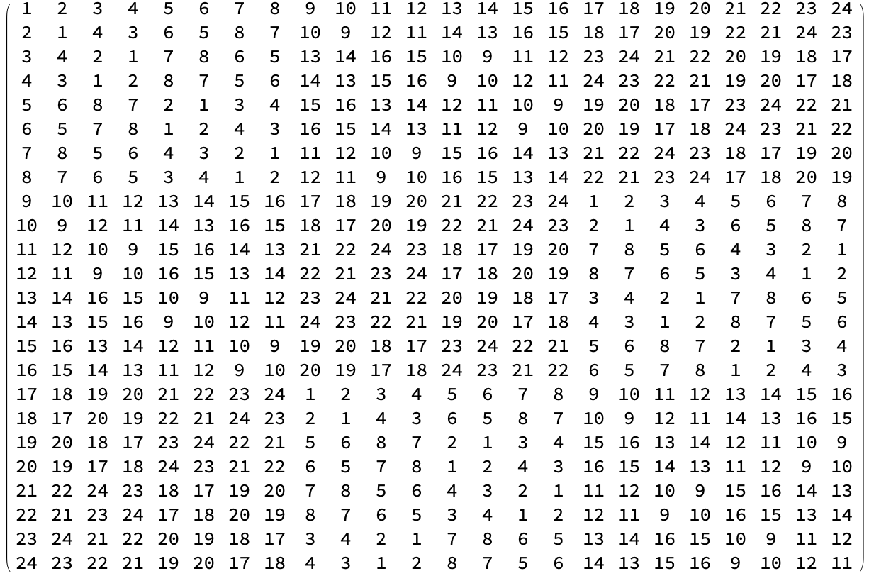

Note how the top left \(8 \times 8\) square contains only the indices from 1 to 8. The \(8 \times 8\) square to the right of it contains only the indices from 9 to 16, and so on: the entire table respects the cosets of \(Q\) and \(K\) because of the order we chose for the elements of \(\text{SL}(2,3).\) All that’s left is to choose colors and visualize the resulting ArrayPlot. The following constructs a list of \(24\) colors for the indices from 1 to 24 so that the first \(8\) are gradually lightening shades of yellow, then next \(8\) are gradually lightening shades of red, and the last \(8\) are gradually lightening shades of blue. Once we have these \(24\) colors in the flat list colorlist, we Blend them to make a ColorFunction that can be passed as an option to ArrayPlot.

colorchoices = {RGBColor["#ffd100"],
		RGBColor["#eb5e28"],
		RGBColor["#457b9d"]};
		
cosetcolors = NestList[Lighter[#, 1/7] &, #, 7] &;

colorlist = Map[cosetcolors, colorchoices] // Flatten;

threecolors = Function[x, Blend[colorlist, x]];

Now all that’s left to do is to color our idxtable using the ColorFunction that we tailor made for this pupose.

ArrayPlot[idxtable, ColorFunction -> threecolors]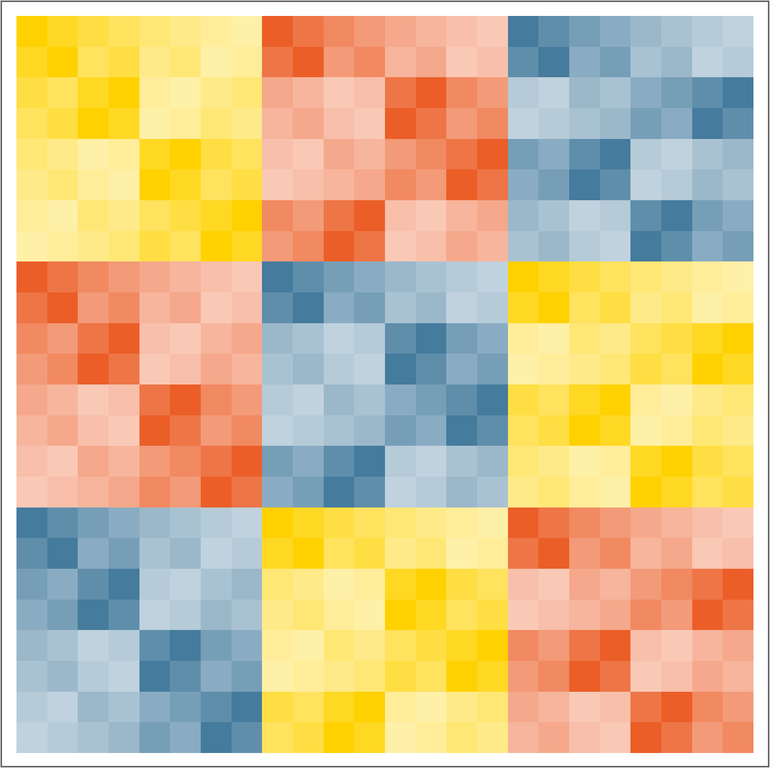

This visualizes the multiplication in \(\text{SL}(2,3)\) in a way that accentuates the flag of normal subgroups

\[\{e\} \trianglelefteq K \trianglelefteq Q \trianglelefteq \text{SL}(2,3)\]

In particular, you can also see Cayley tables for the quotients of \(\text{SL}(2,3)\) by \(Q\) and \(K\): The \(3 \times 3\) grid of red, yellow and blue is the Cayley table for the quotient by \(Q\), while the \(12 \times 12\) grid of \(2\times 2\) squares is the Cayley table for the quotient by \(K\) (which turns out to be isomoprhic to the alternating group \(A_4\)).

You may notice that the top left \(8 \times 8\) square can be viewed as a \(2 \times 2\) grid of \(4 \times 4\) squares, one dark yellow and one light yellow. This is because \(Q\) has normal subgroups that are bigger than \(K\). The one that’s most clearly visible in this Cayley table is \(\{e,-e,i,-i\}\). But while this is normal in \(Q\), it is not normal in \(\text{SL}(2,3)\), which is why the entire Cayley table does not get neatly broken up in to dark and light \(4 \times 4\) squares, and there is no ordering of G that would make that happen because \(\text{SL}(2,3)\) doesn’t have any normal subgroups of index \(6\).